11. Single particle forces (constraints)
espressomd.constraints.Constraint
A Constraint is an immobile surface which can interact with particles via a non-bonded potential, where the distance between the two particles is replaced by the distance of the center of the particle to the surface.
The constraints are identified like a particle via its type particle_type for the
non-bonded interaction. After a type is defined for each constraint one
has to define the interaction of all different particle types with the
constraint using the espressomd.interactions.NonBondedInteractions class.
11.1. Shaped-based constraints
In order to use shapes you first have to import the espressomd.shapes
module. This module provides classes for the different available shapes:
import espressomd.shapes
Shapes define geometries which can be used in ESPResSo either as constraints in particle interactions or as a boundary for a lattice-Boltzmann fluid.
To avoid unexpected behavior make sure all parts of your shape are within the central box since the distance to the shape is calculated only within the central box. If parts of the shape are placed outside of the central box these parts are truncated by the box boundaries. This may or may not be desired as for example in the case of a cylinder without or with cylinder cover.
A shape is instantiated by calling its constructor. If you wanted to create a wall shape you could do:
wall = espressomd.shapes.Wall()
Available shapes are listed below.
11.1.1. Adding shape-based constraints to the system
Usually you want to use constraints based on a shape.
The module espressomd.constraints provides the class
espressomd.constraints.ShapeBasedConstraint:
shape_constraint = espressomd.constraints.ShapeBasedConstraint(shape=my_shape)
In order to add the constraint to the system
invoke the add() method:
system.constraints.add(shape_constraint)
All previously listed shapes can be added to the system constraints
by passing an initialized shape object to add(), returning a constraint object
misshaped = Wall(dist=20, normal=[0.1, 0.0, 1])
myConstraint = system.constraints.add(shape=myShape, particle_type=p_type)
The extra argument particle_type specifies the non-bonded interaction to be used with
that constraint.
There are two additional optional parameters
to fine-tune the behavior of the constraint. If penetrable is set to
True then particles can move through the constraint. In this case the
other option only_positive controls where the particle is subjected to the
interaction potential (see Available options).
If the penetrable option is ignored or is set to False, the
constraint cannot be violated, i.e. no
particle can go through the constraint surface (ESPResSo will exit if any does).
If we wanted to add a non-penetrable pore constraint to our simulation,
we could do the following:
pore = espressomd.shapes.SimplePore(
    axis=[1, 0, 0], length=2, pos=[15, 15, 15], radius=1, smoothing_radius=0.5)
pore_constraint = espressomd.constraints.ShapeBasedConstraint(
    shape=pore, penetrable=False, particle_type=1)
system.constraints.add(pore_constraint)
Interactions between the pore and other particles are then defined as usual (Non-bonded interactions) to prevent particles from crossing the shape surface.
11.1.2. Deleting a constraint
Constraints can be removed in a similar fashion using espressomd.constraints.Constraints.remove()
system.constraints.remove(myConstraint)
This command will delete the specified constraint.
11.1.3. Getting the currently defined constraints
One can iterate through constraints, for example
>>> for c in system.constraints:
...     print(c.shape)
will print the shape information for all defined constraints.
11.1.4. Getting the force on a constraint
espressomd.constraints.ShapeBasedConstraint.total_force()
Returns the force acting on the constraint. Note, however, that this is only due to forces from interactions with particles, not with other constraints. Also, these forces still do not mean that the constraints move, they are just the negative of the sum of forces acting on all particles due to this constraint. Similarly, the total energy does not contain constraint-constraint contributions.
For example the pressure from wall
>>> p = system.constraints[0].total_force()
>>> print(p)
11.1.5. Getting the minimal distance to a constraint
espressomd.constraints.ShapeBasedConstraint.min_dist()
Calculates the smallest distance to all interacting constraints that can be repulsive (wall, cylinder, sphere, rhomboid, pore, slitpore). Negative distances mean that the position is within the area that particles should not access. Helpful to find initial configurations.
11.1.6. Available shapes
Python syntax:
import espressomd from espressomd.shapes import <SHAPE>
system = espressomd.System(box_l=[1, 1, 1])
<SHAPE> can be any of the available shapes.
The surface’s geometry is defined via a few available shapes. The following shapes can be used as constraints.
Warning
When using shapes with concave edges and corners, the fact that a particle only interacts with the closest point on the constraint surface leads to discontinuous force fields acting on the particles. This breaks energy conservation in otherwise symplectic integrators. Often, the total energy of the system increases exponentially.
11.1.6.1. Wall
An infinite plane defined by the normal vector normal
and the distance dist from the origin (in the direction of the normal vector).
The force acts in the direction of the normal.
Note that dist describes the distance from the origin in units of the normal
vector so that the product of dist and normal is a point on the surface.
Therefore negative distances are quite common!
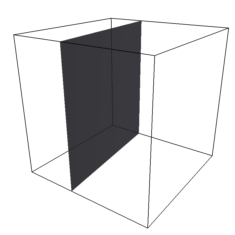
Pictured is an example constraint with a Wall shape created with
wall = Wall(dist=20, normal=[0.1, 0.0, 1])
system.constraints.add(shape=wall, particle_type=0)
For penetrable walls, if the only_positive flag is set to True, interactions
are only calculated if the particle is on the side of the wall in which the
normal vector is pointing.
11.1.6.2. Sphere
A sphere with center center and radius radius.
The direction direction determines the force direction, -1 for inward
and +1 for outward.
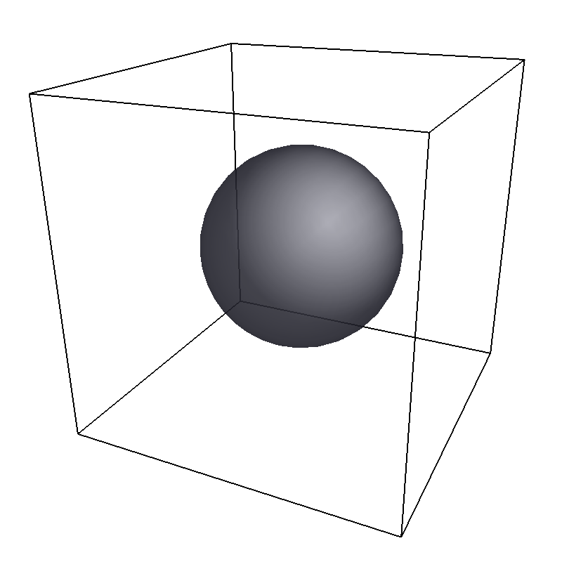
Pictured is an example constraint with a Sphere shape created with
sphere = Sphere(center=[25, 25, 25], radius=15, direction=1)
system.constraints.add(shape=sphere, particle_type=0)
11.1.6.3. Ellipsoid
An ellipsoid with center center, semiaxis a along the symmetry axis and
equatorial semiaxes b. The symmetry axis is aligned parallel to the x-axis.
The direction direction determines the force direction, -1 for inward and +1 for outward.
The distance to the surface is determined iteratively via Newton’s method.
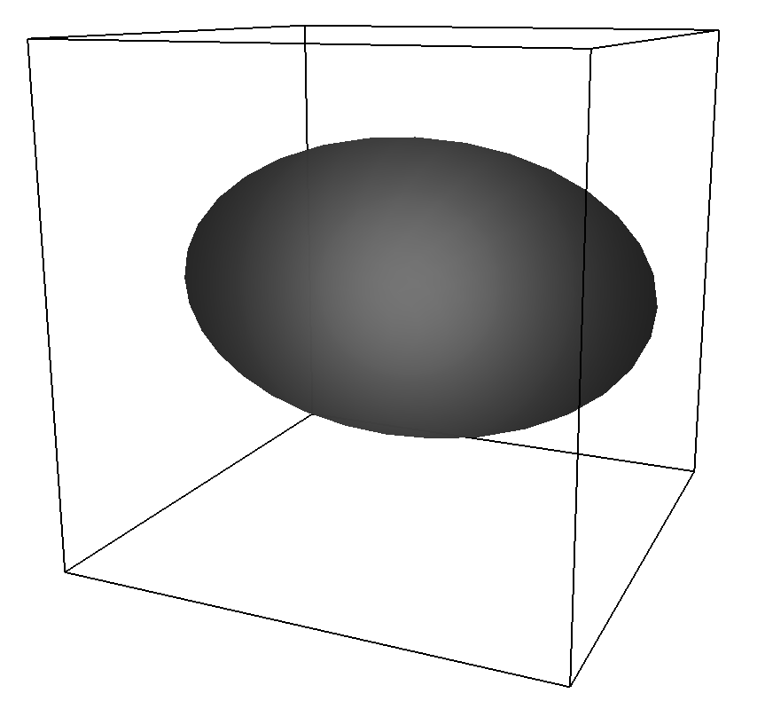
Pictured is an example constraint with an Ellipsoid shape created with
ellipsoid = Ellipsoid(center=[25, 25, 25], a=25, b=15)
system.constraints.add(shape=ellipsoid, particle_type=0)
11.1.6.4. Cylinder
A cylinder with center center, radius radius and length length.
The axis parameter is a vector along the cylinder axis, which is normalized in the program.
The direction direction determines the force direction, -1 for inward and +1 for outward.
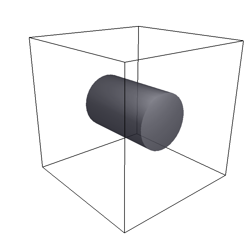
Pictured is an example constraint with a Cylinder shape created with
cylinder = Cylinder(center=[25, 25, 25],
                    axis=[1, 0, 0],
                    direction=1,
                    radius=10,
                    length=30)
system.constraints.add(shape=cylinder, particle_type=0)
11.1.6.5. Rhomboid
A rhomboid or parallelepiped, defined by one corner located at corner
and three adjacent edges, defined by the three vectors connecting the
corner corner with its three neighboring corners: a, b and c.
The direction direction determines the force direction, -1 for inward and +1 for outward.
rhomboid = Rhomboid(corner=[5.0, 5.0, 5.0],
                    a=[1.0, 1.0, 0.0],
                    b=[0.0, 0.0, 1.0],
                    c=[0.0, 1.0, 0.0],
                    direction=1)
system.constraints.add(shape=rhomboid, particle_type=0, penetrable=True)
creates a rhomboid defined by one corner located at [5.0, 5.0, 5.0] and three
adjacent edges, defined by the three vectors connecting the corner with its three neighboring corners, (1,1,0) , (0,0,1) and (0,1,0).
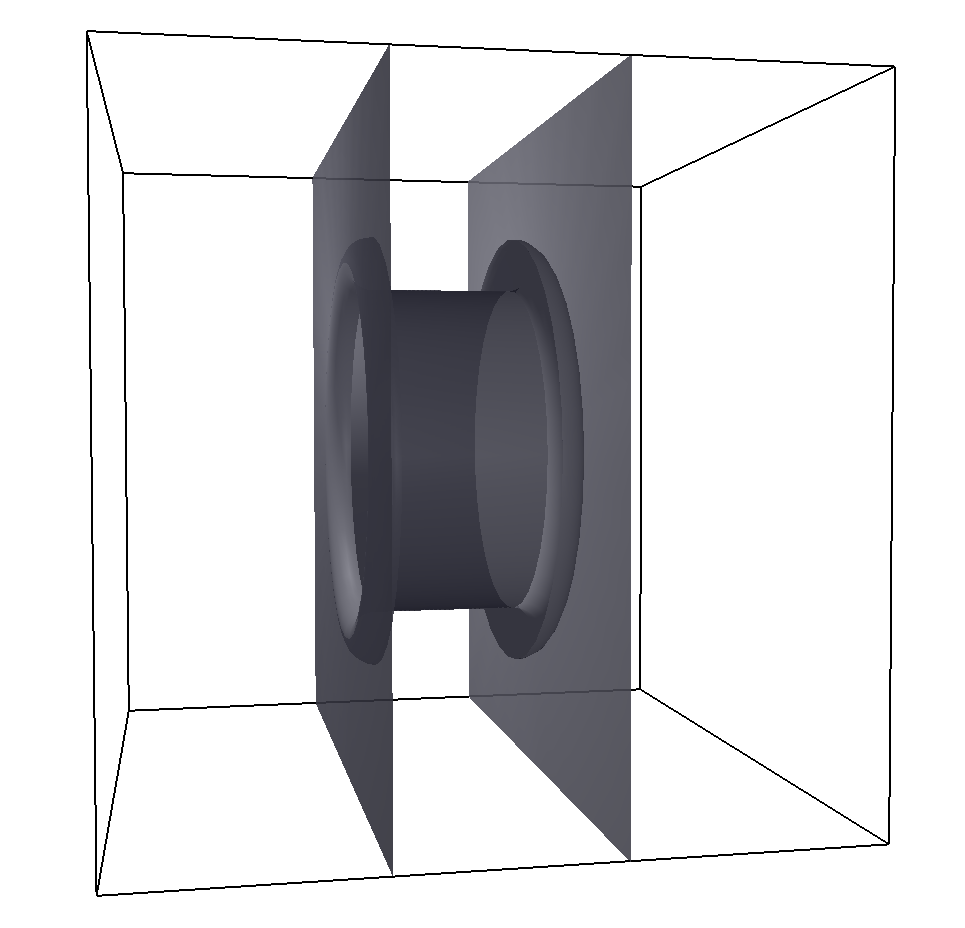
11.1.6.6. SimplePore
Two parallel infinite planes, connected by a cylindrical orifice. The cylinder is connected to the planes by torus segments with an adjustable radius.
Length and radius of the cylindrical pore can be set via the corresponding parameters
length and radius. The parameter center defines the central point of the pore.
The orientation of the pore is given by the vector axis, which points along the cylinder’s symmetry axis.
The pore openings are smoothed with torus segments, the radius of which can be set using the parameter smoothing_radius.
In the OpenGL visualizer, these torus segments are rendered as a half-torus instead of a quarter-torus.
You can safely ignore this visual artifact, in the force/energy calculation, only a quarter-torus is used.
Pictured is an example constraint with a SimplePore shape created with
pore = SimplePore(axis=[1, 0, 0],
                  length=15,
                  radius=12.5,
                  smoothing_radius=2,
                  center=[25, 25, 25])
system.constraints.add(shape=pore, particle_type=0, penetrable=True)
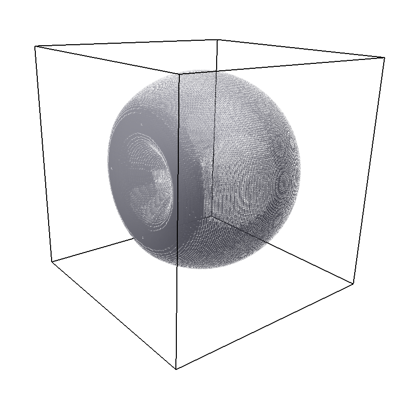
11.1.6.7. Stomatocyte
A stomatocyte-shaped boundary surface.
This command should be used with care.
The position can be any point in the simulation box and is set via the (3,) array_like parameter center.
The orientation of the (cylindrically symmetric) stomatocyte is given by an axis (a (3,) array_like of float),
which points in the direction of the symmetry axis and does not need to be normalized.
Parameters outer_radius, inner_radius, and layer_width specify the
shape of the stomatocyte. Here inappropriate choices of parameters can yield
undesired results, such as discontinuous shapes or NaN values. Always use
values greater than 1 for inner_radius to avoid NaN values.
The width layer_width is used as a scaling parameter.
That is, a stomatocyte given by outer_radius:inner_radius:layer_width = 7:3:1
is half the size of the stomatocyte given by 7:3:2.
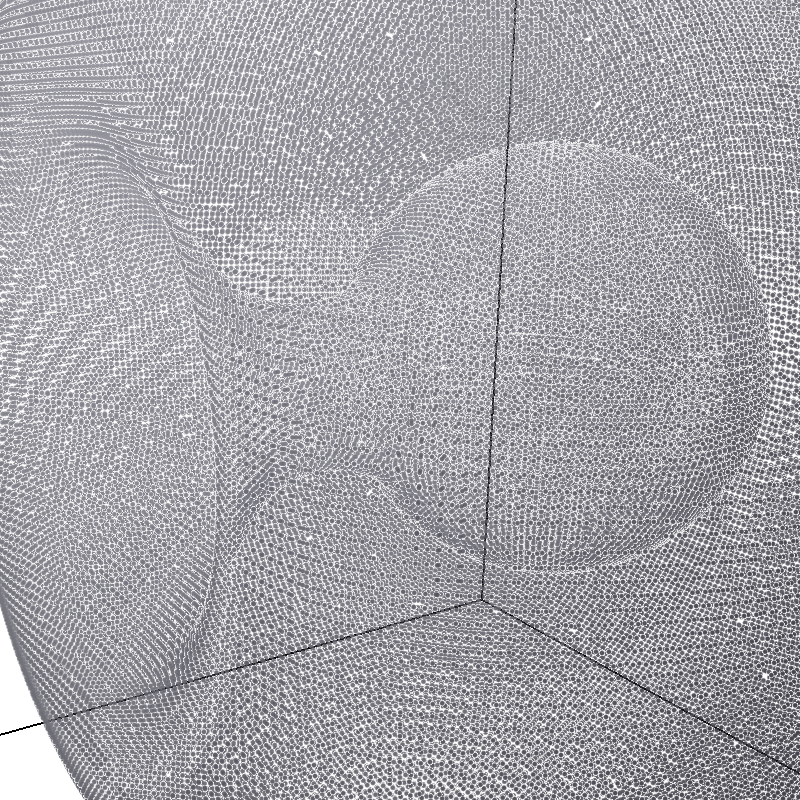
Not all choices of parameters give reasonable values for the shape of the stomatocyte, but the combination 7:3:1 is a good point to start from when trying to modify the shape. If you observe jumps in forces for particles inside the stomatocyte cavity, your parameters are most likely wrong, in which case the OpenGL visualizer will typically fail to draw dots inside the stomatocyte cavity.
Pictured is an example constraint with a Stomatocyte shape (with a closeup of the internal structure) created with
stomatocyte = Stomatocyte(inner_radius=3,
                          outer_radius=7,
                          axis=[1.0, 0.0, 0.0],
                          center=[25, 25, 25],
                          layer_width=3,
                          direction=1)
system.constraints.add(shape=stomatocyte, particle_type=0, penetrable=True)
11.1.6.8. Slitpore
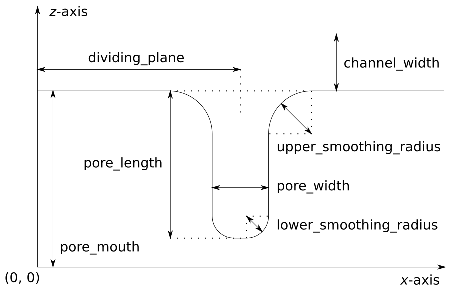
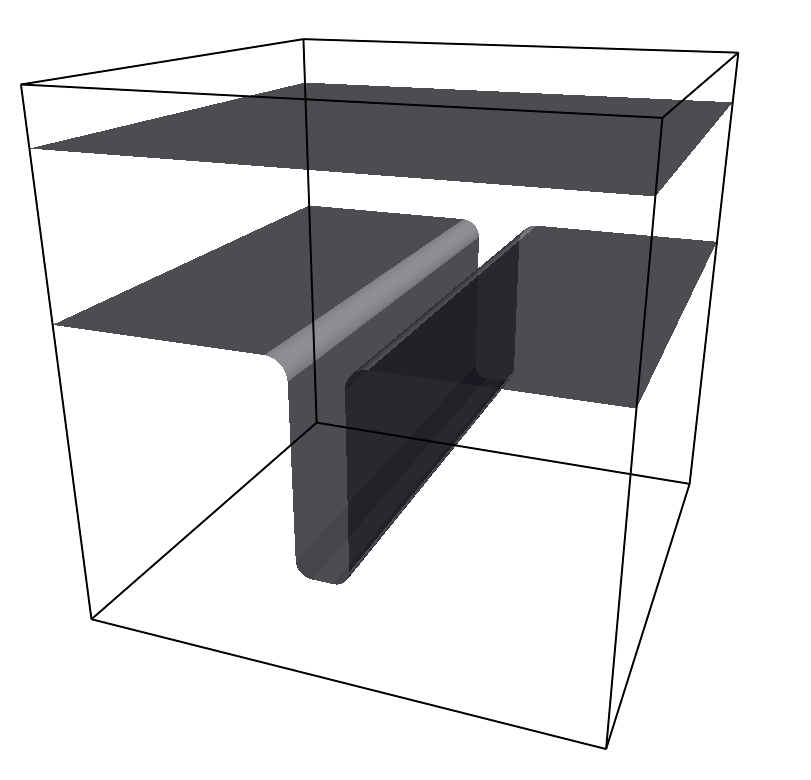
A T-shaped channel that extends in the z-direction. The cross sectional geometry is depicted in Fig. schematic. It is translationally invariant in y direction.
The region is described as a pore (lower vertical part of the “T”-shape) and a channel (upper horizontal part of the “T”-shape).
The parameter channel_width specifies the distance between the top and the plateau edge.
The parameter pore_length specifies the distance between the bottom and the plateau edge.
The parameter pore_width specifies the distance between the two plateau edges, it is the space between the left and right walls of the pore region.
The parameters pore_mouth and dividing_plane specify the location in the z-coordinate resp. x-coordinate of the pore opening.
All the edges are smoothed via the parameters upper_smoothing_radius (for the concave corner at the edge of the plateau region) and lower_smoothing_radius (for the convex corner at the bottom of the pore region).
The meaning of the geometrical parameters can be inferred from the schematic in Fig. slitpore.
Pictured is an example constraint with a Slitpore shape created with
slitpore = Slitpore(channel_width=15,
                    lower_smoothing_radius=1.5,
                    upper_smoothing_radius=2,
                    pore_length=20,
                    pore_mouth=30,
                    pore_width=5,
                    dividing_plane=25)

system.constraints.add(shape=slitpore, particle_type=0, penetrable=True)
11.1.6.9. SpheroCylinder
espressomd.shapes.SpheroCylinder
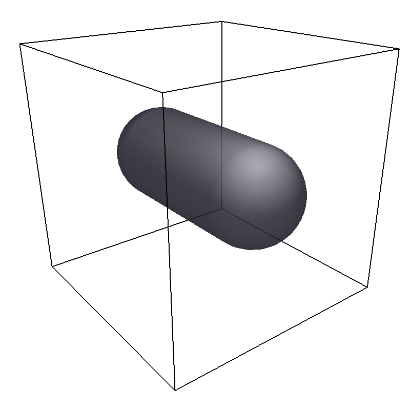
A cylinder capped by hemispheres on both ends. Generates a capsule, pill, or spherocylinder depending on the choice of parameters.
Similar to espressomd.shapes.Cylinder, it is positioned at center and has a radius radius.
The length parameter is the cylinder length, and does not include the contribution from the hemispherical ends.
The axis parameter is a vector along the cylinder axis, which is normalized in the program.
The direction direction determines the force direction, -1 for inward and +1 for outward.
Pictured is an example constraint with a SpheroCylinder shape created with
spherocylinder = SpheroCylinder(center=[25, 25, 25],
                                axis=[1, 0, 0],
                                direction=1,
                                radius=10,
                                length=30)
system.constraints.add(shape=spherocylinder, particle_type=0)
11.1.6.10. Torus
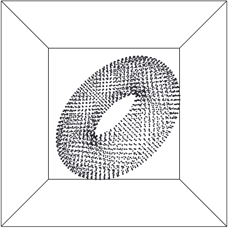
It is positioned at center and has a radius radius with tube radius tube_radius.
The normal parameter is the torus rotation axis, which is normalized in the program.
The direction direction determines the force direction, -1 for inward and +1 for outward.
Pictured is an example constraint with a Torus shape created with
torus = Torus(center=[25, 25, 25], normal=[1, 1, 1],
              direction=1, radius=15, tube_radius=6)
system.constraints.add(shape=torus, particle_type=0)
11.1.6.11. HollowCone
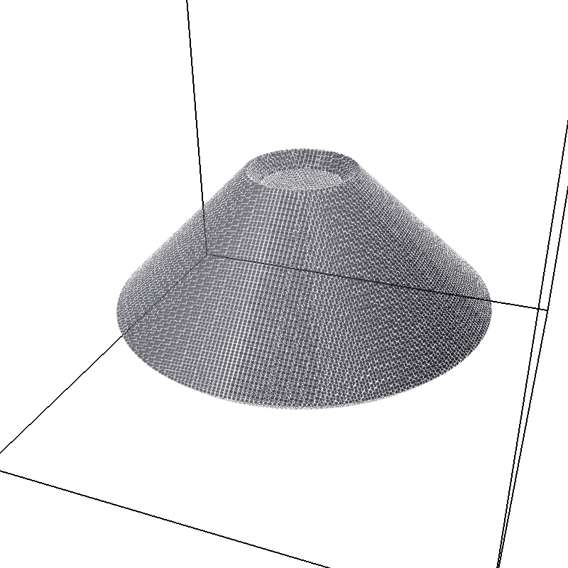
A hollow cone with round corners.
The parameters inner_radius and outer_radius specifies the two radii .
The parameter opening_angle specifies the opening angle of the cone (in radians, between 0 and \(\pi/2\) ), and thus also determines the length.
The orientation of the (cylindrically symmetric) cone is specified with the parameter axis (a (3,) array_like of float),
which points in the direction of the symmetry axis, and does not need to be normalized.
The position is specified via the (3,) array_like center and can be any point in the simulation box.
The width specifies the width.
This shape supports the direction parameter, +1 for outward and -1 for inward.
Pictured is an example constraint with a HollowCone shape created with
hollowcone = HollowCone(inner_radius=5,
                        outer_radius=20,
                        opening_angle=np.pi/4.0,
                        axis=[1.0, 0.0, 0.0],
                        center=[25, 25, 25],
                        width=2,
                        direction=1)
system.constraints.add(shape=hollowcone, particle_type=0, penetrable=True)
11.1.7. Available options
There are some options to help control the behaviour of shaped-based
constraints. Some of the options, like direction need to be specified for
the shape espressomd.shapes, and some options are specified for the
constraint espressomd.constraints.ShapeBasedConstraint. We will
discuss them together in this section in the context of a specific example.
The direction option typically specifies which volumes are inside versus
outside the shape. Consider a constraint based on the sphere shape. If one
wishes to place particles inside the sphere, one would usually use
direction=-1, if one wishes to place particles outside, one would use
direction=1. In this example, we place a sphere centre at position
(25,0,0). A particle is continuously displaced on the x-axis in order to probe
the effect of different options. For this, we need to first define a repulsive
interaction between the probe and the constraint.
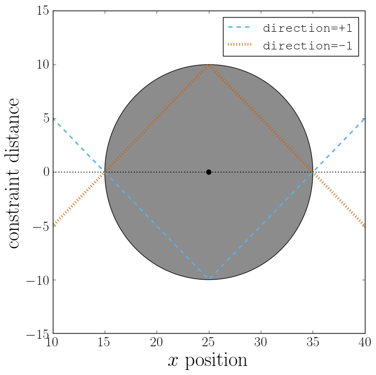
The plot below demonstrates how the distance between the probe and the
constraint surface is calculated when the distance option is toggled
between direction=1 and direction=-1. In the plot, a schematic of a
circle centered at x=25 is used to represent the spherical constraint.
When the option direction=1 is used for the sphere shape, positive
distances are measured whenever the particle is outside the sphere and negative
distances are measured whenever the particle is inside the sphere. Conversely,
when the option direction=-1 is used for the sphere shape, negative
distances are measured whenever the particle is outside the sphere and positive
distances are measured whenever the particle is inside the sphere. In other
words, this option helps defines the sign of the normal surface vector.
For now, this may not sound useful but it can be practical when used with
together with constraint options such as penetrable or only_positive.
In the former case, using non-penetrable surfaces with penetrable=False will
cause ESPResSo to throw an error is any distances between interacting particles and
constraints are found to be negative. This can be used to stop a simulation if
for one reason or another particles end up in an unwanted location.
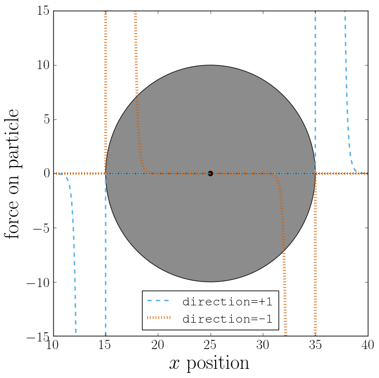
The only_positive constraint option is used to define if a force should be
applied to a particle that has a negative distance. For example, consider the
same probe particle as in the previous case. The plot below shows the particle
force with only_positive=True. Notice that when the distance is negative,
forces are not applied at all to the particle. Thus the constraint surface is
either purely radially outwards (when direction=1) or radially inwards
(when direction=-1). Note that in both cases the constraint was set to be
penetrable with penetrable=True or else the simulation would crash whenever
the particle was found in any location that yields a negative distance.
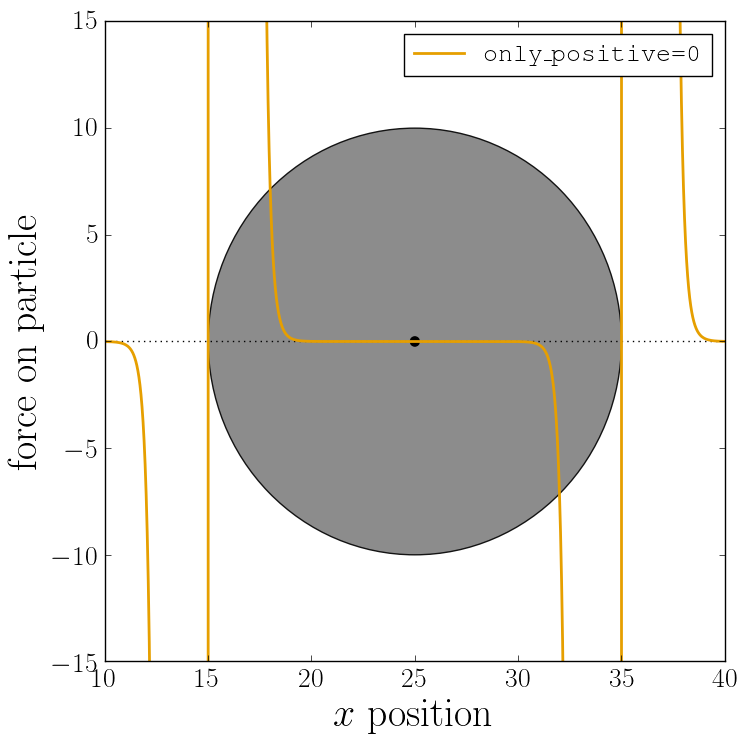
The next figure shows what happens if we turn off the only_positive flag by
setting only_positive=False. In this case the particle is pushed radially
inward if it is inside the sphere and radially outward if it is outside. As
with the previous example, the constraint was set to be penetrable for this to
make sense.
Most shapes have a clear interpretation of what is inside versus outside with
the exception of a planar wall. For this, there is no direction option, but
the normal vector of the wall points in the direction that is considered to
yield positive distances. Outside their use in constraints, shapes can also be
used as a way to define LB boundary nodes. In this case, negative distances
define nodes which are part of a boundary (please refer to Using shapes as lattice-Boltzmann boundary).
11.2. External Fields
There is a variety of external fields, which differ by how their values are obtained and how they couple to particles.
11.2.1. Constant fields
These are fields that are constant in space or simple linear functions of the position. The available fields are:
A detailed description can be found in the class documentation.
Please be aware of the fact that a constant per-particle force can be
set via the ext_force property of the particles and is not provided
here.
11.2.2. Interpolated Force and Potential fields
The values of these fields are obtained by interpolating table data, which has to be provided by the user. The fields differ by how they couple to particles, for a detailed description see their respective class documentation.
