5. Setting up particles

5.1. Overview of the relevant Python classes

For understanding this chapter, it is helpful to be aware of the Python classes provided by ESPResSo to interact with particles:

• ParticleHandle provides access to a single particle in the simulation.

• ParticleList provides access to all particles in the simulation

• ParticleSlice provides access to a subset of particles in the simulation identified by a list of ids or an instance of slice or range.

In almost no case have these classes to be instantiated explicitly by the user. Rather, access is provided via the system part attribute. The details are explained in the following sections.

5.2. Adding particles

In order to add particles to the system, call ParticleList.add():

import espressomd
system = espressomd.System(box_l=[10., 10., 10.])
p = system.part.add(pos=[1., 1., 1.], type=0)

This command adds a single particle to the system with properties given as arguments, and it returns an instance of ParticleHandle, which will be used to access properties of the newly created particle. The pos property is required, all other properties are optional. All available particle properties are members of ParticleHandle.

Note that the instances of ParticleHandle returned by ParticleList.add() are handles for the live particles in the simulation, rather than offline copies. Changing their properties will affect the simulation.

It is also possible to add several particles at once:

import numpy as np
new_parts = system.part.add(pos=np.random.random((10, 3)) * box_length)

If several particles are added at once, an instance of ParticleSlice is returned.

Particles are identified via their id property. A unique id is given to them automatically. Alternatively, you can assign an id manually when adding them to the system:

system.part.add(pos=[1., 2., 3.], id=system.part.highest_particle_id + 1)

The id provides an alternative way to access particles in the system. To retrieve the handle of the particle with id 5, call:

p = system.part.by_id(5)

5.3. Accessing particle properties

Particle properties can be accessed like any class member.

For example, to print the particle’s current position, call:

print(p.pos)

5.4. Modifying particle properties

Similarly, the position can be set:

p.pos = [1., 2.5, 3.]

Not all properties are writeable. For example, properties that are automatically derived from other properties are read-only attributes.

Please note that changing a particle property will not affect the ghost particles until after the next integration loop. This can be an issue for certain methods like espressomd.system.System.distance() which use the old ghost information, while other methods like particle-based analysis tools and espressomd.cell_system.CellSystem.get_neighbors() update the ghost information before calculating the observable.

5.4.1. Vectorial properties

For vectorial particle properties, component-wise manipulation like p.pos[0] = 1 or in-place operators like += or *= are not allowed and raise an exception. This behavior is inherited, so the same applies to pos after pos = p.pos. If you want to use a vectorial property for further calculations, you should explicitly make a copy e.g. via pos = numpy.copy(p.pos).

5.5. Deleting particles

Particles can be easily deleted in Python using particle ids or ranges of particle ids. For example, to delete all particles of type 1, run:

system.part.select(type=1).remove()

To delete all particles, use:

system.part.clear()

5.6. Iterating over particles and pairs of particles

You can iterate over all particles or over a subset of particles (see Interacting with groups of particles) as follows:

for p in system.part:
    print(p.pos)

for p in system.part.select(type=1):
    print(p.pos)

You can iterate over all pairs of particles using:

for pair in system.part.pairs():
    print(pair[0].id, pair[1].id)

5.7. Exclusions

Particles can have an exclusion list of all other particles where non-bonded interactions are ignored. This is typically used in atomistic simulations, where nearest and next nearest neighbor interactions along a chain of bonded particles have to be omitted since they are included in the bonding potentials. Exclusions do not apply to the short range part of electrostatics and magnetostatics methods, e.g. to P3M.

To create exclusions for particles pairs 0 and 1:

system.part.by_id(0).add_exclusion(1)

To delete the exclusion:

system.part.by_id(0).delete_exclusion(1)

The current list of exclusions is accessible in the exclusions property.

5.8. Rotational degrees of freedom and particle anisotropy

When the feature ROTATION is compiled in, particles not only have a position, but also an orientation that changes with an angular velocity. A torque on a particle leads to a change in angular velocity depending on the particles rotational inertia. The property rinertia has to be specified as the three eigenvalues of the particles rotational inertia tensor. Even if the particle rotational inertia is isotropic, the rotation state can be important if, e.g., the particle carries a dipole or is an active particle.

The rotational degrees of freedom are integrated using a velocity Verlet scheme. The implementation is based on a quaternion representation of the particle orientation and described in [Omelyan, 1998] with quaternion components indexing made according to the formalism \(q = a + b\mathbf{i} + c\mathbf{j} + d\mathbf{k}\) [Allen and Tildesley, 2017].

When the Langevin thermostat is enabled, the rotational degrees of freedom are also thermalized.

Whether or not rotational degrees of freedom are propagated, is controlled on a per-particle and per-axis level, where the axes are the Cartesian axes of the particle in its body-fixed frame. It is important to note that starting from version 4.0 and unlike in earlier versions of ESPResSo, the particles’ rotation is disabled by default. In this way, just compiling in the ROTATION feature no longer changes the physics of the system.

The rotation of a particle is controlled via the rotation property. E.g., the following code adds a particle with rotation enabled around the x-axis of its body frame:

import espressomd
system = espressomd.System(box_l=[1, 1, 1])
system.part.add(pos=(0, 0, 0), rotation=(True, False, False))

The rotational state of a particle is stored as a quaternion in the quat property. For a value of (1,0,0,0), the body and space frames coincide. When setting up a particle, its orientation state is by default aligned with the space frame of the box. If your particles have a rotational symmetry, you can set up the particle direction (the symmetry axis) using the director property. Note that then you have no control over the initial rotation angle around the symmetry axis. If your particles are anisotropic in all three directions, you can either set the quat attribute directly, or (recommended) set up all particle properties in the box frame and then use rotate to rotate the particle to the desired state before starting the simulation.

Notes:

• The space-frame direction of the particle’s z-axis in its body frame is accessible through the director property.

• Any other vector can be converted from body to space fixed frame using the ParticleHandle.convert_vector_body_to_space() method.

• When DIPOLES are compiled in, the particles dipole moment is always co-aligned with the z-axis in the body-fixed frame.

• Changing the particles dipole moment and director will re-orient the particle such that its z-axis in space frame is aligned parallel to the given vector. No guarantees are made for the other two axes after setting the director or the dipole moment.

The following particle properties are related to rotation:

• dip

• director

• ext_torque

• gamma_rot

• gamma_rot

• omega_body

• omega_lab

• quat

• rinertia

• rotation

• torque_lab

5.9. Virtual sites

Virtual sites are particles, the positions and velocities of which are not obtained by integrating an equation of motion. Rather, their coordinates are obtained from the position (and orientation) of one or more other particles. In this way, rigid arrangements of particles can be constructed and a particle can be placed in the center of mass of a set of other particles. Virtual sites can interact with other particles in the system by means of interactions. Forces are added to them according to their respective particle type. Before the next integration step, the forces accumulated on a virtual site are distributed back to those particles, from which the virtual site was derived.

There are different schemes for virtual sites, described in the following sections. To switch the active scheme, the system virtual_sites property can be used:

import espressomd
import espressomd.virtual_sites

system = espressomd.System(box_l=[1, 1, 1])
system.virtual_sites = espressomd.virtual_sites.VirtualSitesRelative(have_quaternion=False)
# or
system.virtual_sites = espressomd.virtual_sites.VirtualSitesOff()

By default, espressomd.virtual_sites.VirtualSitesOff is selected. This means that virtual particles are not touched during integration. The have_quaternion parameter determines whether the quaternion of the virtual particle is updated (useful in combination with the vs_quat property of the virtual particle which defines the orientation of the virtual particle in the body fixed frame of the related real particle).

5.9.1. Rigid arrangements of particles

The relative implementation of virtual sites allows for the simulation of rigid arrangements of particles. It can be used, for extended dipoles and raspberry-particles, but also for more complex configurations. Position and velocity of a virtual site are obtained from the position and orientation of exactly one non-virtual particle, which has to be placed in the center of mass of the rigid body. Several virtual sites can be related to one and the same non-virtual particle. The position of the virtual site is given by

\[\vec{x_v} =\vec{x_n} +O_n (O_v \vec{E_z}) d,\]

where \(\vec{x_n}\) is the position of the non-virtual particle, \(O_n\) is the orientation of the non-virtual particle, \(O_v\) denotes the orientation of the vector \(\vec{x_v}-\vec{x_n}\) with respect to the non-virtual particles body fixed frame and \(d\) the distance between virtual and non-virtual particle. In words: The virtual site is placed at a fixed distance from the non-virtual particle. When the non-virtual particle rotates, the virtual sites rotates on an orbit around the non-virtual particles center.

To use this implementation of virtual sites, activate the feature VIRTUAL_SITES_RELATIVE. Furthermore, an instance of VirtualSitesRelative has to be set as the active virtual sites scheme (see above). To set up a virtual site:

1. Place the particle to which the virtual site should be related. It needs to be in the center of mass of the rigid arrangement of particles you create:

   import espressomd
   import espressomd.virtual_sites
   
   system = espressomd.System(box_l=[10., 10., 10.])
   system.virtual_sites = espressomd.virtual_sites.VirtualSitesRelative()
   p1 = system.part.add(pos=[1., 2., 3.])
   

2. Place a particle at the desired relative position, make it virtual and relate it to the first particle:

   rel_offset = [1., 0., 0.]
   p2 = system.part.add(pos=p1.pos + rel_offset)
   p2.vs_auto_relate_to(p1)
   

   This will set the virtual attribute on particle p2 to True.

3. Repeat the previous step with more virtual sites, if desired.

4. To update the positions of all virtual sites, call:

   system.integrator.run(0, recalc_forces=True)
   

Please note:

• The relative position of the virtual site is defined by its distance from the non-virtual particle, the id of the non-virtual particle and a quaternion which defines the vector from non-virtual particle to virtual site in the non-virtual particles body-fixed frame. This information is saved in the virtual site’s vs_relative attribute. Take care, not to overwrite it after using vs_auto_relate.

• Virtual sites can not be placed relative to other virtual sites, as the order in which the positions of virtual sites are updated is not guaranteed. Always relate a virtual site to a non-virtual particle placed in the center of mass of the rigid arrangement of particles.

• In case you know the correct quaternions, you can also setup a virtual site using its vs_relative and virtual attributes.

• In a simulation on more than one CPU, the effective cell size needs to be larger than the largest distance between a non-virtual particle and its associated virtual sites. To this aim, when running on more than one core, you need to set the system’s min_global_cut attribute to this largest distance. An error is generated when this requirement is not met.

• If the virtual sites represent actual particles carrying a mass, the inertia tensor of the non-virtual particle in the center of mass needs to be adapted.

• The presence of rigid bodies constructed by means of virtual sites adds a contribution to the scalar pressure and pressure tensor.

5.9.2. Inertialess lattice-Boltzmann tracers

espressomd.virtual_sites.VirtualSitesInertialessTracers

When this implementation is selected, the virtual sites follow the motion of a lattice-Boltzmann fluid (both, CPU and GPU). This is achieved by integrating their position using the fluid velocity at the virtual sites’ position. Forces acting on the virtual sites are directly transferred as force density onto the lattice-Boltzmann fluid, making the coupling free of inertia. The feature stems from the implementation of the Immersed Boundary Method for soft elastic objects, but can be used independently.

For correct results, the LB thermostat has to be deactivated for virtual sites:

system.thermostat.set_lb(kT=0, act_on_virtual=False)

Please note that the velocity attribute of the virtual particles does not carry valid information for this virtual sites scheme.

5.10. Interacting with groups of particles

Groups of particles are addressed using ParticleSlice objects. Usually, these objects do not have to be instantiated by the user. There are several ways to retrieve a particle slice:

• By calling ParticleList.add()

  When adding several particles at once, a particle slice is returned instead of a particle handle.

• By calling ParticleList.by_ids()

  It is also possible to get a slice containing particles of specific ids, e.g.:

  system.part.by_ids([1, 4, 3])
  

  would contain the particles with ids 1, 4, and 3 in that specific order.

• By calling ParticleList.all()

  You can get a slice containing all particles using:

  system.part.all()
  

• By calling ParticleList.select()

  This is useful to filter out particles with distinct properties, e.g.:

  slice1 = system.part.select(type=0, q=1)
  slice2 = system.part.select(lambda p: p.pos[0] < 0.5)
  

Properties of particle slices can be accessed just like with single particles. A list of all values is returned:

print(system.part.all().q)

A particle slice can be iterated over, see Iterating over particles and pairs of particles.

Setting properties of slices can be done by

• supplying a single value that is assigned to each entry of the slice, e.g.:

  system.part.by_ids(range(10)).ext_force = [1, 0, 0]
  

• supplying an array of values that matches the length of the slice which sets each entry individually, e.g.:

  system.part.by_ids(range(3)).ext_force = [[1, 0, 0], [2, 0, 0], [3, 0, 0]]
  

For list properties that have no fixed length like exclusions or bonds, some care has to be taken. There, single value assignment also accepts lists/tuples just like setting the property of an individual particle. For example:

system.part.by_id(0).exclusions = [1, 2]

would both exclude short-range interactions of the particle pairs 0 <-> 1 and 0 <-> 2. Similarly, a list can also be assigned to each entry of the slice:

system.part.by_ids(range(2,4)).exclusions = [0, 1]

This would exclude interactions between 2 <-> 0, 2 <-> 1, 3 <-> 0 and 3 <-> 1. Now when it is desired to supply an array of values with individual values for each slice entry, the distinction can no longer be done by the length of the input, as slice length and input length can be equal. Here, the nesting level of the input is the distinctive criterion:

system.part.by_ids(range(2,4)).exclusions = [[0, 1], [0, 1]]

The above code snippet would lead to the same exclusions as the one before. The same accounts for the bonds property by interchanging the integer entries of the exclusion list with the tuple (bond, partners).

You can select a subset of particles via using the select method. For example you can obtain a list of particles with charge -1 via using

system.part.select(q=-1)

For further information on how to use selections see espressomd.particle_data.ParticleList.select().

5.11. Create particular particle configurations

5.11.1. Setting up polymer chains

If you want to have polymers in your system, you can use the function espressomd.polymer.linear_polymer_positions() to determine suitable positions.

Required arguments are the desired number of polymers n_polymers, the number of monomers per polymer chain beads_per_chain, and the parameter bond_length, which determines the distance between adjacent monomers within the polymer chains. Determining suitable particle positions pseudo-randomly requires the use of a pseudo-random number generator, which has to be seeded. This seed is therefore also a mandatory parameter.

The function espressomd.polymer.linear_polymer_positions() returns a three-dimensional numpy array, namely a list of polymers containing the positions of monomers (x, y, z). A quick example of how to set up polymers:

import espressomd
import espressomd.polymer
import espressomd.interactions

system = espressomd.System([50, 50, 50])
fene = espressomd.interactions.FeneBond(k=10, d_r_max=2)
system.bonded_inter.add(fene)
polymer_positions = espressomd.polymer.linear_polymer_positions(
    n_polymers=10, beads_per_chain=25, bond_length=0.9, seed=23)

for positions in polymer_positions:
    monomers = system.part.add(pos=positions)
    previous_part = None
    for part in monomers:
        if not previous_part is None:
            part.add_bond((fene, previous_part))
        previous_part = part

If there are constraints present in your system which you want to be taken into account when creating the polymer positions, you can set the optional boolean parameter respect_constraint=True. To simulate excluded volume while drawing the polymer positions, a minimum distance between all particles can be set via min_distance. This will also respect already existing particles in the system. Both when setting respect_constraints and choosing a min_distance trial positions are pseudo-randomly chosen and only accepted if the requested requirement is fulfilled. Otherwise, a new attempt will be made, up to max_tries times per monomer and if this fails max_tries per polymer. The default value is max_tries=1000. Depending on the total number of beads and constraints, this value may need to be adapted. If determining suitable polymer positions within this limit fails, a runtime error is thrown.

Note that the distance between adjacent monomers during the course of the simulation depends on the applied potentials. For fixed bond length please refer to the Rattle Shake algorithm[Andersen, 1983]. The algorithm is based on Verlet algorithm and satisfy internal constraints for molecular models with internal constraints, using Lagrange multipliers.

5.11.2. Setting up diamond polymer networks

espressomd.polymer.setup_diamond_polymer() creates a diamond-structured polymer network with 8 tetra-functional nodes connected by \(2 \times 8\) polymer chains of length MPC with the system box as the unit cell. The box therefore has to be cubic. The diamond command creates 16*MPC+8 many particles which are connected via the provided bond type (the term plus 8 stems from adding 8 nodes which are connecting the chains). Chain monomers are placed at constant distance to each other along the vector connecting network nodes. The distance between monomers is system.box_l[0]*(0.25 * sqrt(3))/(MPC + 1), which should be taken into account when choosing the connecting bond. The starting particle id, the charges of monomers, the frequency of charged monomers in the chains as well as the types of the node particles, the charged and the uncharged chain particles can be set via keyword arguments, see espressomd.polymer.setup_diamond_polymer().

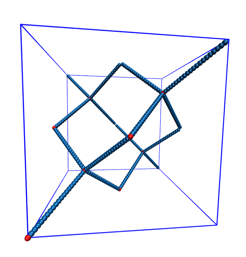
Diamond-like polymer network with MPC=15.

For simulating compressed or stretched gels, the function espressomd.system.System.change_volume_and_rescale_particles() may be used.

5.12. Particle number counting feature

Note

Do not use these methods with the espressomd.collision_detection module since the collision detection may create or delete particles without the particle number counting feature being aware of this. Therefore the espressomd.reaction_methods module may not be used with the collision detection.

Knowing the number of particles of a certain type in simulations where particle numbers can fluctuate is of interest. Particle ids can be stored in a map for each individual type:

import espressomd
system = espressomd.System(box_l=[1, 1, 1])
system.setup_type_map([_type])
system.number_of_particles(_type)

If you want to keep track of particle ids of a certain type you have to initialize the method by calling

system.setup_type_map([_type])

After that the system will keep track of particle ids of that type. Keeping track of particles of a given type is not enabled by default since it requires memory. The keyword number_of_particles as argument will return the number of particles which have the given type. For counting the number of particles of a given type you could also use ParticleList.select()

import espressomd
system = espressomd.System(box_l=[1, 1, 1])
system.part.add(pos=[1, 0, 0], type=0)
system.part.add(pos=[0, 1, 0], type=0)
system.part.add(pos=[0, 0, 1], type=2)
print(len(system.part.select(type=0)))
print(len(system.part.select(type=2)))

However calling select(type=type) results in looping over all particles, which is slow. In contrast, the system number_of_particles() method can return the number of particles with that type.

5.13. Self-propelled swimmers

Note

If you are using this feature, please cite [de Graaf et al., 2016].

See also

swimming

5.13.1. Langevin swimmers

import espressomd
system = espressomd.System(box_l=[1, 1, 1])
system.part.add(pos=[1, 0, 0], swimming={'f_swim': 0.03})

This enables the particle to be self-propelled in the direction determined by its quaternion. For setting the particle’s quaternion see quat. The self-propulsion speed will relax to a constant velocity, that is specified by v_swim. Alternatively it is possible to achieve a constant velocity by imposing a constant force term f_swim that is balanced by friction of a (Langevin) thermostat. The way the velocity of the particle decays to the constant terminal velocity in either of these methods is completely determined by the friction coefficient. You may only set one of the possibilities v_swim or f_swim as you cannot relax to constant force and constant velocity at the same time. Note that there is no real difference between v_swim and f_swim, since the latter may always be chosen such that the same terminal velocity is achieved for a given friction coefficient.

5.13.2. Lattice-Boltzmann swimmers

import espressomd
system = espressomd.System(box_l=[1, 1, 1])
system.part.add(pos=[2, 0, 0], rotation=[1, 1, 1], swimming={
    'f_swim': 0.01, 'mode': 'pusher', 'dipole_length': 2.0})

For an explanation of the parameters v_swim and f_swim see the previous item. In lattice-Boltzmann self-propulsion is less trivial than for regular MD, because the self-propulsion is achieved by a force-free mechanism, which has strong implications for the far-field hydrodynamic flow field induced by the self-propelled particle. In ESPResSo only the dipolar component of the flow field of an active particle is taken into account. This flow field can be generated by a pushing or a pulling mechanism, leading to change in the sign of the dipolar flow field with respect to the direction of motion. You can specify the nature of the particle’s flow field by using one of the modes: pusher or puller. You will also need to specify a dipole_length which determines the distance of the source of propulsion from the particle’s center. Note that you should not put this distance to zero; ESPResSo (currently) does not support mathematical dipole flow fields.

You may ask: “Why are there two methods v_swim and f_swim for the self-propulsion using the lattice-Boltzmann algorithm?” The answer is straightforward. When a particle is accelerating, it has a monopolar flow-field contribution which vanishes when it reaches its terminal velocity (for which there will only be a dipolar flow field). The major difference between the above two methods is that with v_swim the flow field only has a monopolar moment and only while the particle is accelerating. As soon as the particle reaches a constant speed (given by v_swim) this monopolar moment is gone and the flow field is zero! In contrast, f_swim always, i.e., while accelerating and while swimming at constant force possesses a dipolar flow field.