Electrokinetics part 2: electroosmotic flow

Table of contents

1. Introduction
2. Analytical solution
3. Setting up the simulation
4. Comparison to the analytical solution
5. Comparison to pressure-driven flow

This is the second of the three parts of the electrokinetics tutorial:

• Part 1 (advection-diffusion): advection-diffusion of a neutral tracer species in a prescribed two-dimensional flow field.
• Part 2 (this notebook): an electrolyte confined in a slit pore and driven by an external electric field.
• Part 3 (reactive flow): an irreversible bulk reaction in the turbulent wake behind an array of cylinders.

This notebook is self-contained, but it assumes that you are familiar with the basic setup of an electrokinetics simulation as introduced in part 1.

1. Introduction

The electrokinetics feature of ESPResSo describes the motion of potentially charged chemical species solvated in a fluid on a continuum level. The governing equations are the Poisson-Nernst-Planck equations coupled to the incompressible Navier-Stokes equation,

$$ \begin{aligned} \partial_{t} n_{i} &= - \vec{\nabla} \cdot \vec{j}_{i} \\ \vec{j}_{i} &= - D_{i} \vec{\nabla} n_{i} - \frac{z_{i} e}{k_{B} T} n_{i} \vec{\nabla} \phi + n_{i} \vec{u} \\ \Delta \phi &= \frac{1}{4 \pi \varepsilon_{0} \varepsilon_{\mathrm{r}}} \sum_{i} z_{i} e n_{i} \\ \rho (\partial_{t} \vec{u} + (\vec{u} \cdot \vec{\nabla}) \vec{u}) &= - \vec{\nabla} p + \eta \Delta \vec{u} + \sum_{i} \frac{k_{B} T}{D_{i}} \vec{j}_{i} + \vec{f}_{\mathrm{ext}} \\ \vec{\nabla} \cdot \vec{u} &= 0, \end{aligned} $$

with the ion densities $n_{i}$, the density fluxes $\vec{j}_{i}$, the diffusion coefficients $D_{i}$, the valencies $z_{i}$, the electrostatic potential $\phi$, the fluid velocity $\vec{u}$ and the dynamic viscosity $\eta$. In contrast to part 1, we now keep the electrostatic Poisson equation, since the species we simulate carries a charge.

The system in this part of the tutorial is a simple slit pore, as shown in Figure 1. It consists of an infinite plate capacitor with an electrolytic solution trapped in between the plates. The plates of the capacitor carry a constant surface charge and the counterions are solvated in the liquid.

Charge attraction will cause the ions to accumulate near the surfaces, forming a characteristic ion density profile, which can be calculated analytically using the Poisson-Boltzmann equation. Since the system has translational symmetry in the directions parallel to the plates, the equations for parallel and orthogonal direction decouple. This means that applying an external electric field in a direction parallel to the plates will not change the distribution of the ions along the orthogonal direction. It will however cause motion of the ions and consequently the fluid: the characteristic flow profile of electroosmotic flow.

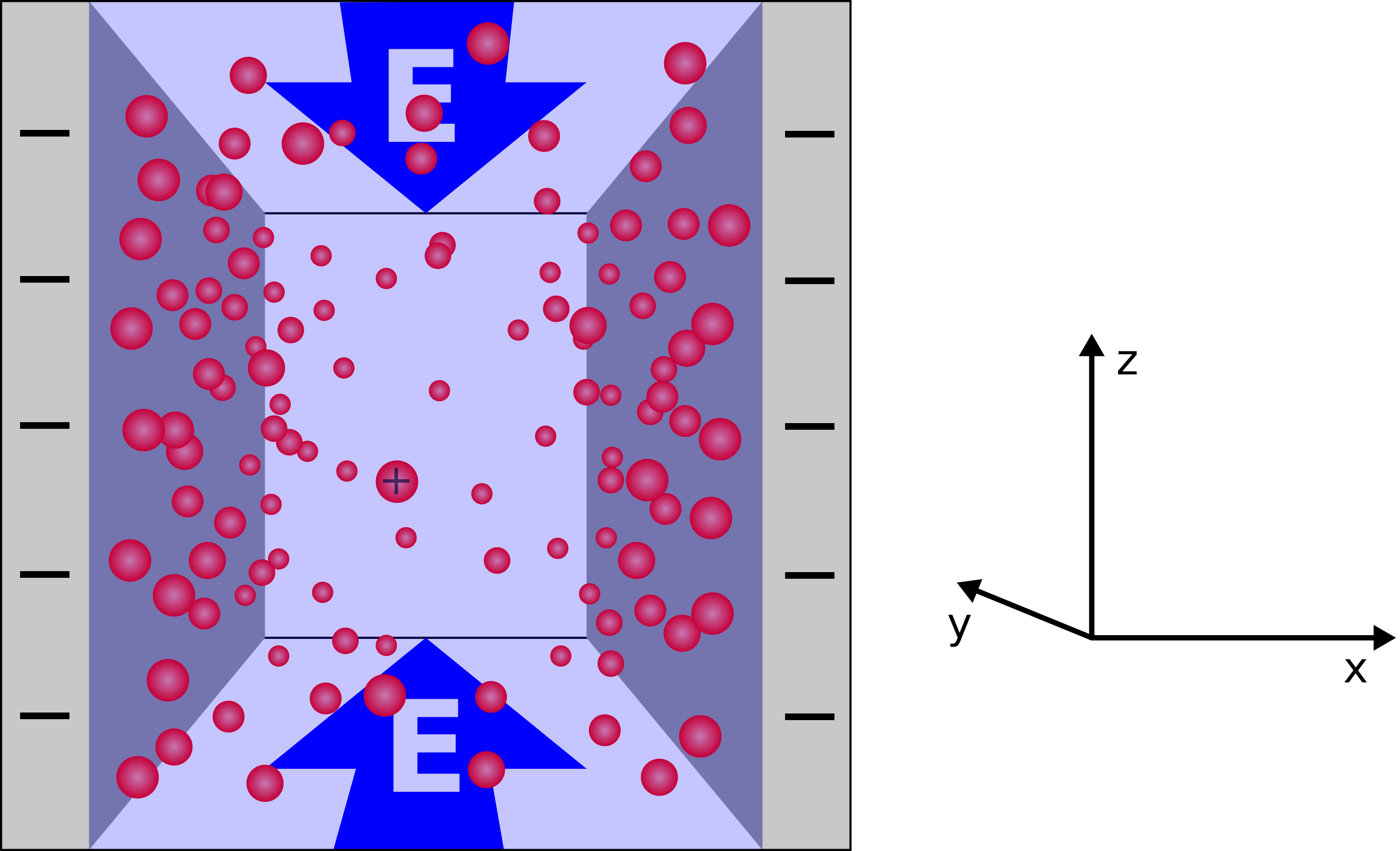
Figure 1: Slit pore system and coordinate system used for the analytical calculations.

</center> </figure>

2. Analytical solution

Due to the symmetries of the system, it effectively reduces to a 1D problem along the orthogonal axis. The system can be described by the Poisson-Boltzmann equation:

$$ \partial_{x}^2 \phi(x) = \frac{1}{\varepsilon_{0} \varepsilon_{\mathrm{r}}} \sum_{i} z_{i} e n_{i}(x) \exp \left( -\frac{z_{i} e \phi(x)}{k_{\mathrm{B}} T} \right) $$

where $x$ is the normal-direction of the plates. Since we will only simulate a single ion species, the counterions, the sum only has a single summand. The solution for the potential is then given by:

$$ \phi(x) = -\frac{k_{B}T}{z e} \log \left[ \frac{C^2 \varepsilon_{0} \varepsilon_{\mathrm{r}}}{2 k_{B}T } \cos^{-2} \left( \frac{z e C}{2 k_{B} T} x \right) \right], \qquad \text{with } \left\| \frac{z e C}{2 k_{B} T} \right\| < \frac{\pi}{2}, $$

where $C$ is an integration constant that is to be determined by the boundary conditions. The ion density follows then from the potential as

$$ n(x) = \frac{C^2 \varepsilon_{0} \varepsilon_{\mathrm{r}}}{2 k_{B}T} \cos^{-2} \left( \frac{z e C}{2 k_{B} T} x \right). $$

To find the integration constant we use the fact that the total system has to be charge neutral, i.e., the total charge on the plates is counterbalanced by the counterions. This leads to the following equation

$$ C \tan \left( \frac{z e d}{4 k_{B} T} C \right) = - \frac{e^2}{\varepsilon_{0} \varepsilon_{\mathrm{r}}} \sigma, $$

where $\sigma$ is the surface charge density of the plates. This is a transcendental equation, which must be solved numerically to find $C$.

The electric field is applied in the $y$-direction, parallel to the plates. Fluid flow is described by the incompressible Navier-Stokes equation, which due to the symmetries of the system reduces to the one-dimensional problem

$$ \frac{\partial^2 v_{y}(x)}{\partial x^2} = - \frac{\varepsilon_{0} \varepsilon_{\mathrm{r}} z e E C^2}{2 k_{B}T \eta} \cos^{-2}\left( \frac{q C}{2 k_{B} T} x \right). $$

This equation can be solved analytically and the solution is given by

$$ v_{y}(x) = \frac{2 \varepsilon_{0} \varepsilon_{\mathrm{r}} k_{B} T E}{\eta z e} \log \left( \frac{\cos \left( \displaystyle\frac{z e C}{2 k_{B} T} x \right)}{\cos \left( \displaystyle\frac{z e C}{2 k_{B} T} \frac{d}{2} \right)} \right), $$

where $d$ denotes the distance between the two plates. Finally, the shear stress of this problem is given by

$$ \sigma(x) = \mu \frac{\partial v_{y}(x)}{\partial x} $$

3. Setting up the simulation

We start by importing the necessary packages and defining the parameters. Note that this part of the tutorial needs the FFT-based Poisson solver, which is only available if ESPResSo was built with the WALBERLA_FFT feature.

import espressomd
import espressomd.lb
import espressomd.electrokinetics
import espressomd.shapes

espressomd.assert_features(["WALBERLA", "WALBERLA_FFT"])

import tqdm.auto as tqdm
import numpy as np

import scipy.optimize

import matplotlib.pyplot as plt

plt.rcParams.update({'font.size': 14})

AGRID = 1.0
TAU = 1.0
KT = 2.0
PERMITTIVITY = 0.28
DIFFUSION_COEFFICIENT = 0.25
VALENCY = 1.0
VISCOSITY_DYNAMIC = 0.5
DENSITY_FLUID = 1.0
SURFACE_CHARGE_DENSITY = -0.05
EXT_FORCE_DENSITY = [0.0, 0.01, 0.0]

SINGLE_PRECISION = False

padding = 1
WIDTH = 126
BOX_L = [(WIDTH + 2 * padding) * AGRID, 1, 1]

RUN_TIME = 200

The two directions parallel to the plates are only one lattice cell wide. Together with the periodic boundary conditions of ESPResSo this realizes the translational symmetry of the infinite plate capacitor. The two extra cells given by padding are the cells that will hold the surface charge of the plates.

system = espressomd.System(box_l=BOX_L)
system.cell_system.skin = 0.4
system.time_step = TAU

We set up the LB method exactly as in part 1, so we simply give the code here. The only subtlety is the viscosity: LBFluid expects the kinematic viscosity $\nu = \eta / \rho$, whereas the analytical expressions above (and the parameter VISCOSITY_DYNAMIC) are given in terms of the dynamic viscosity $\eta$. As in part 1 the fluid is not thermalized, so kT keeps its default value of 0.

lattice = espressomd.lb.Lattice(agrid=AGRID, n_ghost_layers=1)

viscosity_kinematic = VISCOSITY_DYNAMIC / DENSITY_FLUID
lbf = espressomd.lb.LBFluid(lattice=lattice, density=DENSITY_FLUID,
                            kinematic_viscosity=viscosity_kinematic,
                            tau=TAU, single_precision=SINGLE_PRECISION)
system.lb = lbf

Since our species are going to carry a charge now, we need to solve the full electrostatic problem. In contrast to part 1, where the placeholder EKNone was enough, we now have to specify an actual solver.

Exercise 1

• Set up a Poisson solver for the electrostatic interaction and use it to create an instance of the EKContainer.
• Attach the container to system.ekcontainer.

Hints:

• Use an EKFFT object as the Poisson solver, with permittivity PERMITTIVITY.
• Both objects take tau=TAU; the solver also takes single_precision=SINGLE_PRECISION.

# SOLUTION CELL
eksolver = espressomd.electrokinetics.EKFFT(lattice=lattice, permittivity=PERMITTIVITY,
                                            tau=TAU, single_precision=SINGLE_PRECISION)
system.ekcontainer = espressomd.electrokinetics.EKContainer(tau=TAU, solver=eksolver)

To simulate the system, we will use two different ion species. The first are the counterions that are propagated in the fluid. Creating them works just like the EKSpecies in part 1, except that they now carry a charge (valency) and feel an external electric field, so we give the code directly.

ekspecies = espressomd.electrokinetics.EKSpecies(
    lattice=lattice, density=0.0, kT=KT, diffusion=DIFFUSION_COEFFICIENT,
    valency=VALENCY, advection=True, friction_coupling=True,
    ext_efield=EXT_FORCE_DENSITY, single_precision=SINGLE_PRECISION, tau=TAU)
system.ekcontainer.add(ekspecies)

The second species is used to represent the surface charge on the plates. This is a concept we have not seen yet: instead of modeling the charged plates explicitly, we store their charge as an EKSpecies that is held fixed in space. It therefore must neither diffuse nor be advected, and it must not exert a friction force on the fluid.

Exercise 2

• Create the immobile wall charge species ekwallcharge with valency -VALENCY and add it to system.ekcontainer.

Hints:

• Use the same constructor arguments as for the counterions above (lattice, tau=TAU, kT=KT, density=0.0, single_precision=SINGLE_PRECISION), but make the species immobile: diffusion=0., advection=False, friction_coupling=False and ext_efield=[0, 0, 0].

# SOLUTION CELL
ekwallcharge = espressomd.electrokinetics.EKSpecies(
    lattice=lattice, density=0.0, kT=KT, diffusion=0.,
    valency=-VALENCY, advection=False, friction_coupling=False,
    ext_efield=[0, 0, 0], single_precision=SINGLE_PRECISION, tau=TAU)
system.ekcontainer.add(ekwallcharge)

Now we set the initial conditions for the ion densities. The counterions will be initialized with a homogeneous distribution, excluding the cells used as boundaries. The surface charge density is homogeneously distributed in the boundary cells.

density_counterions = -2.0 * SURFACE_CHARGE_DENSITY / VALENCY / WIDTH
ekspecies[padding:-padding, :, :].density = density_counterions

ekspecies[:padding, :, :].density = 0.0
ekspecies[-padding:, :, :].density = 0.0

ekwallcharge[:padding, :, :].density = -SURFACE_CHARGE_DENSITY / VALENCY / padding
ekwallcharge[-padding:, :, :].density = -SURFACE_CHARGE_DENSITY / VALENCY / padding

The FFT-based Poisson solver assumes periodic boundary conditions, which are only compatible with an overall charge-neutral system. Let us verify that the initial condition satisfies this constraint.

total_charge = sum(species.valency * np.sum(species[:, :, :].density) * AGRID**3
                   for species in system.ekcontainer)
print(f"total charge in the simulation box: {total_charge:.2e}")

total charge in the simulation box: 2.78e-17

We now have to specify the boundary conditions. For this, we use ESPResSo's shapes.

wall_left = espressomd.shapes.Wall(normal=[1, 0, 0], dist=padding)
wall_right = espressomd.shapes.Wall(normal=[-1, 0, 0], dist=-(padding + WIDTH))

At both of them we specify no-flux and zero-density boundary conditions for the counterions. Furthermore, we set a no-slip boundary condition for the fluid.

Exercise 3

At both walls, set

• no-flux boundary conditions for the counterions (ekspecies),
• zero-density boundary conditions for the counterions,
• no-slip boundary conditions for the fluid (lbf).

Hints:

• Use the shapes defined above and add_boundary_from_shape for EK species and LB fluids.
• The boundary type is selected with the boundary_type argument, which takes either FluxBoundary or DensityBoundary. A flux boundary condition takes a vector as value, a density boundary condition a scalar.
• The wall charge species must not get boundary conditions, otherwise the density we just placed in the boundary cells would be erased.

# SOLUTION CELL
for wall in (wall_left, wall_right):
    ekspecies.add_boundary_from_shape(
        shape=wall, value=[0., 0., 0.],
        boundary_type=espressomd.electrokinetics.FluxBoundary)
    ekspecies.add_boundary_from_shape(
        shape=wall, value=0.0,
        boundary_type=espressomd.electrokinetics.DensityBoundary)
    lbf.add_boundary_from_shape(shape=wall, velocity=[0., 0., 0.])

4. Comparison to the analytical solution

Now we can finally integrate the system and extract the ion density profile, the fluid velocity profile as well as the pressure tensor profile.

for i in tqdm.trange(80):
    system.integrator.run(RUN_TIME)

mid_y = int(system.box_l[1] / (2 * AGRID))
mid_z = int(system.box_l[2] / (2 * AGRID))
density_eof = ekspecies[padding:-padding, mid_y, mid_z].density
velocity_eof = lbf[padding:-padding, mid_y, mid_z].velocity[:, 1]
pressure_tensor_eof = lbf[padding:-padding, mid_y, mid_z].pressure_tensor[:, 0, 1]

positions = (np.arange(len(density_eof)) - WIDTH / 2 + 0.5) * AGRID

For comparison, we calculate the analytic solution. The integration constant $C$ is obtained by numerically solving the transcendental equation from section 2.

def transcendental_equation(c, distance, kT, sigma, valency, permittivity) -> float:
    elementary_charge = 1.0
    return c * np.tan(valency * elementary_charge * distance / (4 * kT) * c) + sigma / permittivity


solution = scipy.optimize.fsolve(func=transcendental_equation, x0=0.001, args=(
    WIDTH, KT, SURFACE_CHARGE_DENSITY, VALENCY, PERMITTIVITY))


def eof_density(x, c, permittivity, elementary_charge, valency, kT):
    return c**2 * permittivity / (2 * kT) / (np.cos(valency * elementary_charge * c / (2 * kT) * x))**2


def eof_velocity(x, c, permittivity, elementary_charge, valency, kT, ext_field, distance, viscosity):
    return 2 * kT * ext_field * permittivity / (viscosity * elementary_charge * valency) * np.log(
        np.cos(valency * elementary_charge * c / (2 * kT) * x) / np.cos(valency * elementary_charge * c / (2 * kT) * distance / 2))


def eof_pressure_tensor(x, c, elementary_charge, valency, kT, ext_field, permittivity):
    return permittivity * ext_field * c * np.tan(valency * elementary_charge * c / (2 * kT) * x)

analytic_density_eof = eof_density(x=positions, c=solution, permittivity=PERMITTIVITY,
                                   elementary_charge=1.0, valency=VALENCY, kT=KT)
analytic_velocity_eof = eof_velocity(x=positions, c=solution, permittivity=PERMITTIVITY,
                                     elementary_charge=1.0, valency=VALENCY, kT=KT,
                                     ext_field=EXT_FORCE_DENSITY[1], distance=WIDTH,
                                     viscosity=VISCOSITY_DYNAMIC)
analytic_pressure_tensor_eof = eof_pressure_tensor(x=positions, c=solution, elementary_charge=1.0,
                                                   valency=VALENCY, kT=KT,
                                                   ext_field=EXT_FORCE_DENSITY[1],
                                                   permittivity=PERMITTIVITY)

fig1 = plt.figure(figsize=(16, 4.5))
fig1.suptitle("electroosmotic flow")

ax = fig1.add_subplot(131)
ax.plot(positions, density_eof, "o", mfc="none", markevery=0.015, label="simulation")
ax.plot(positions, analytic_density_eof, label="analytic")
ax.set_xlabel("x-position")
ax.set_ylabel("Counter-ion density")
ax.ticklabel_format(axis="y", style="scientific", scilimits=(0, 0))
ax.legend(loc="best")

ax = fig1.add_subplot(132)
ax.plot(positions, velocity_eof, "o", mfc="none", markevery=0.015, label="simulation")
ax.plot(positions, analytic_velocity_eof, label="analytic")
ax.set_xlabel("x-position")
ax.set_ylabel("Fluid velocity")
ax.ticklabel_format(axis="y", style="scientific", scilimits=(0, 0))
ax.legend(loc="best")

ax = fig1.add_subplot(133)
ax.plot(positions, pressure_tensor_eof, "o", mfc="none", markevery=0.015, label="simulation")
ax.plot(positions, analytic_pressure_tensor_eof, label="analytic")
ax.set_xlabel("x-position")
ax.set_ylabel("Fluid shear stress xz")
ax.ticklabel_format(axis="y", style="scientific", scilimits=(0, 0))
ax.legend(loc="best")

plt.tight_layout()
plt.show()

In the plots one can see that the analytic solution for the electroosmotic flow matches the simulation very well.

5. Comparison to pressure-driven flow

We can compare electroosmotic flow to pressure-driven flow. For this, we turn off the external electric field and enable a constant external force density on the fluid instead. The magnitude of the body force is much smaller than the electric field used before, because now the whole fluid is driven instead of only the charged boundary layers.

EXT_FORCE_DENSITY = [0.0, 0.000004, 0.0]

Exercise 4

The ion distribution is determined by the problem orthogonal to the plates and is therefore independent of how the flow parallel to the plates is driven. Replace the electrophoretic driving by a homogeneous body force on the fluid:

• Switch off the external electric field acting on the counterions.
• Apply the newly defined EXT_FORCE_DENSITY to the LB fluid.

Hints:

• The external field of a species is stored in EKSpecies.ext_efield, the body force of the fluid in LBFluid.ext_force_density.
• Both properties can simply be overwritten on the existing objects; there is no need to re-create them.

# SOLUTION CELL
ekspecies.ext_efield = [0.0, 0.0, 0.0]
lbf.ext_force_density = EXT_FORCE_DENSITY

for i in tqdm.trange(70):
    system.integrator.run(RUN_TIME)

density_pressure = ekspecies[padding:-padding, mid_y, mid_z].density
velocity_pressure = lbf[padding:-padding, mid_y, mid_z].velocity[:, 1]
pressure_tensor_pressure = lbf[padding:-padding, mid_y, mid_z].pressure_tensor[:, 0, 1]

The analytic solution for pressure-driven flow between two infinite parallel plates is known as the Poiseuille flow.

def pressure_velocity(x, distance, ext_field, viscosity):
    return ext_field / (2 * viscosity) * (distance**2 / 4 - x**2)


def pressure_pressure_tensor(x, ext_field):
    return ext_field * x

analytic_velocity_pressure = pressure_velocity(x=positions, distance=WIDTH,
                                               ext_field=EXT_FORCE_DENSITY[1],
                                               viscosity=VISCOSITY_DYNAMIC)
analytic_pressure_tensor_pressure = pressure_pressure_tensor(x=positions,
                                                             ext_field=EXT_FORCE_DENSITY[1])

fig1 = plt.figure(figsize=(16, 4.5))
fig1.suptitle("pressure-driven flow")

ax = fig1.add_subplot(131)
ax.plot(positions, density_pressure, "o", mfc="none", markevery=0.015, label="simulation")
ax.plot(positions, analytic_density_eof, label="analytic")
ax.set_xlabel("x-position")
ax.set_ylabel("counter-ion density")
ax.ticklabel_format(axis="y", style="scientific", scilimits=(0, 0))
ax.legend(loc="best")

ax = fig1.add_subplot(132)
ax.plot(positions, velocity_pressure, "o", mfc="none", markevery=0.015, label="simulation")
ax.plot(positions, analytic_velocity_pressure, label="analytic")
ax.set_xlabel("x-position")
ax.set_ylabel("fluid velocity")
ax.ticklabel_format(axis="y", style="scientific", scilimits=(0, 0))
ax.legend(loc="best")

ax = fig1.add_subplot(133)
ax.plot(positions, pressure_tensor_pressure, "o", mfc="none", markevery=0.015, label="simulation")
ax.plot(positions, analytic_pressure_tensor_pressure, label="analytic")
ax.set_xlabel("x-position")
ax.set_ylabel("fluid shear stress xz")
ax.ticklabel_format(axis="y", style="scientific", scilimits=(0, 0))
ax.legend(loc="best")

plt.tight_layout()
plt.show()

As one can again see, the body force on the fluid did not alter the ion density profile. However, because the force now applies homogeneously on the whole fluid, the flow profile looks parabolic.

To see the difference between the two types of flows, we plot the simulation data together in one plot.

fig1 = plt.figure(figsize=(16, 4.5))
fig1.suptitle("electroosmotic vs. pressure-driven flow comparison")

ax = fig1.add_subplot(131)
ax.plot(positions, density_eof, "o", mfc="none", ms=4, markevery=0.015, label="eof")
ax.plot(positions, density_pressure, "o", mfc="none", markevery=0.015, label="pressure")
ax.set_xlabel("x-position")
ax.set_ylabel("counter-ion density")
ax.ticklabel_format(axis="y", style="scientific", scilimits=(0, 0))
ax.legend(loc="best")

ax = fig1.add_subplot(132)
ax.plot(positions, velocity_eof, "o", mfc="none", markevery=0.015, label="eof")
ax.plot(positions, velocity_pressure, "o", mfc="none", markevery=0.015, label="pressure")
ax.set_xlabel("x-position")
ax.set_ylabel("fluid velocity")
ax.ticklabel_format(axis="y", style="scientific", scilimits=(0, 0))
ax.legend(loc="best")

ax = fig1.add_subplot(133)
ax.plot(positions, pressure_tensor_eof, "o", mfc="none", markevery=0.015, label="eof")
ax.plot(positions, pressure_tensor_pressure, "o", mfc="none", markevery=0.015, label="pressure")
ax.set_xlabel("x-position")
ax.set_ylabel("fluid shear stress xz")
ax.ticklabel_format(axis="y", style="scientific", scilimits=(0, 0))
ax.legend(loc="best")

plt.tight_layout()
plt.show()

Looking at the fluid velocity plot, one can see that the electroosmotic flow profile flattens significantly faster towards the center of the channel when compared to the pressure-driven flow. The reason for this is the accumulation of the counterion density towards the oppositely charged plates. Here, the driving electric field causes the highest force on the fluid, which decays towards the center of the channel. In contrast, the Poiseuille flow is driven by a constant, uniform driving force.

In part 3 we will add chemical reactions between several species and study them in a turbulent flow field.