Machine Learned Interatomic Potentials (MLIP) with ESPResSo

In this tutorial, you'll learn how to train and deploy a machine-learned interatomic potential (MLIP) with ESPResSo. We'll be using the apax MLIP framework [1],[2]. In the first part, we will make ourselves familiar with atomistic simulations of water in ESPResSo, which is the system we will study here. Part two will address the MLIP in detail, before we use it in part three within ESPResSo and benchmark it against experiments and the classical water simulations.

Part 1: Atomistic simulations of water with TIP4P model

We begin with a classical MD simulation of liquid water using the TIP4P/2005 model [3]. This model is one of the most widely used classical force fields in computational chemistry and material science for accurately representing the structual and thermodynamic properties of water.

The primary objectives of this part of tutorial are:

  • To learn how to set up and run an atomistic simulation of water molecules using the TIP4P model
  • To explore the structure of liquid water by computing and analyzing the radial distribution function (RDF)
  • To establish a reference for later comparison with simulations based on MLIP

This atomistic approach provides a valuable baseline against with more modern methods, i.e. MLIP, can be evaluated in terms of both accuracy and performance.

We will now import the necessary ESPResSo features and external modules and proceed to setup the system.

In [1]:
import espressomd
import espressomd.observables
import numpy as np
import pandas as pd
import scipy.constants
import tqdm.auto as tqdm
import pint
import matplotlib.pyplot as plt
%matplotlib inline
plt.rcParams.update({'font.size': 14})
espressomd.assert_features(["LENNARD_JONES", "P3M", "VIRTUAL_SITES_RELATIVE"])
/usr/lib/python3/dist-packages/tqdm/auto.py:21: TqdmWarning: IProgress not found. Please update jupyter and ipywidgets. See https://ipywidgets.readthedocs.io/en/stable/user_install.html
  from .autonotebook import tqdm as notebook_tqdm

Simulation units

In this simulation, energies are expressed in $k_{B}T$ with T = 298.15 K, distances in nanometers, masses in atomic units and charge in unit charge. Physical quantities are managed by the pint unit registry.

In [2]:
# Simulation units:
# * energy: kT
# * mass: atomic mass unit
# * length: nm
# * charge: unit chage

u = pint.UnitRegistry()
Q_ = u.Quantity

# --- Fundamental constants (CODATA exact where defined) ---
eps0 = Q_(scipy.constants.epsilon_0, "farad/meter")  # vacuum permittivity
NA = Q_(6.02214076e23, "1 / mole")  # Avogadro constant
kB = Q_(scipy.constants.k, "joule/kelvin")  # Boltzmann constant
T = Q_(298.15, "kelvin")  # temperature

u.define(f"kT = {(kB * T).to("joule")}")  # kT
u.define(f"e = {scipy.constants.e} * coulomb")  # elementary charge

# System size
L = (25 * u.angstrom).m_as(u.nm)

These constants are defined in order to convert all simulation parameters to dimensionless quantities.

TIP4P model

The TIP4P model is a classical, rigid water model designed to simulate the water molecular behaviour in MD and Monte Carlo simulations. Unlike simpler models, such as TIP3P or SPC, which use three interaction sites, the water molecule consists of four fixed interaction sites arranged as a rigid body in the TIP4P model:

  • Two hydrogen atoms, each with a positive partial charge q_H.
  • One oxygen atom, which participates in Lennard-Jones interactions but carries no charge.
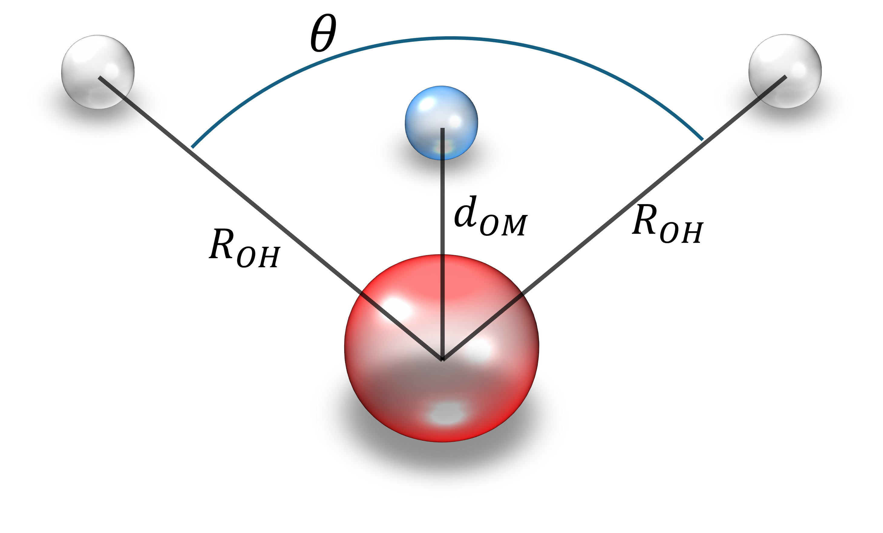
  • A massless dummy site (called the M site) located slightly offset, d_OM, from the oxygen atom along the bisector of the H-O-H angle. The negative partial charge of the molecule, q_M, is assigned to this M site.

This fixed geometry, maintained through rigid constraints, allows efficient simulations with larger time steps. More importantly, the placement of the negative charge at the M site enhances the electrostatic representation, particularly improving the dipole and quadrupole moments of the water molecule.

Among its variants, TIP4P/2005 [3] is particularly well-regarded for accurately key structural and thermodynamic properties of water. While slightly more computationally demanding than three-site model, TIP4P/2005 offers a strong balance between physical realism and performance.

TIP4P

Therefore, we set parameters for moleculary geometry and Lennard-Jones potential following TIP4P/2005.

Exercise:

  • Set following parameters:
    • OO_SIGMA: The sigma for Lennard-Jones interactions between oxygen
    • OO_EPSILON: The (dimensionless) interaction strength epsilon for Lennard-Jones interactions between oxygen
    • R_OH: The distance between oxygen and hydrogen
    • theta: H-O-H angle
    • d_OM: The distance between oxygen and the M site
    • q_H: a partial charge for hydrogen
    • q_M: a partial charge for the M site

Hint:

  • All parameters are wrriten in the paper [3].
In [3]:
# SOLUTION CELL
# --- TIP4P/2005 Lennard-Jones (oxygen site) ---
OO_SIGMA = (3.1589 * u.angstrom).m_as(u.nm)
OO_EPSILON = (Q_(93.2, "kelvin") / T).to("dimensionless").magnitude

# --- TIP4P/2005 geometry ---
R_OH = (0.9572 * u.angstrom).m_as(u.nm)
theta = np.radians(104.52)
d_OM = (0.1546 * u.angstrom).m_as(u.nm)
q_H = (+0.5564 * u.e).m_as(u.e)
q_M = (-1.1128 * u.e).m_as(u.e)

The geometry of water molecule is defined according to TIP4P/2005.

Exercise:

  • Specify the geometry of water molecule for TIP4P/2005 by setting following parameters (as NumPy arrays):
    • O_loc: Position of oxygen
    • H1_loc: Position of hydrogen 1
    • H2_loc: Position of hydrogen 2
    • M_loc: Position of the M site

Hint:

  • Only the relative positions need to be defined. For simplicity, you can place all atoms in the same plane. For example O_loc at the origin and H1_loc on the x-axis. Then place the other atoms according to the model description.
In [4]:
# SOLUTION CELL
O_loc = np.array([0.0, 0.0, 0.0])
H1_loc = np.array([R_OH, 0.0, 0.0])
H2_loc = np.array([R_OH * np.cos(theta), R_OH * np.sin(theta), 0.0])
M_loc = np.array([d_OM * np.cos(theta / 2.0), d_OM * np.sin(theta / 2.0), 0.0])

Other parameters are adjusted to match actual physical constants.

In [5]:
# masses
O_MASS = (15.9994 * u.u).m_as(u.u)
H_MASS = (1.008 * u.u).m_as(u.u)
# center of mass position
COM = (O_MASS * O_loc + H_MASS * (H1_loc + H2_loc)) / (O_MASS + 2 * H_MASS)

# number density of water molecules
WATER_DENSITY = Q_(0.997, "g/cm^3")
TIP4P_MASS = Q_(O_MASS + 2 * H_MASS, "g/mole")
RHO_N = (WATER_DENSITY / TIP4P_MASS * NA).to("1/nm^3").magnitude

COULOMB_CONSTANT = 1 / (4 * np.pi * eps0.to("e^2/kT/nm")).magnitude

Setup system

We set system size L=2.5 nm, and the number of water molecule n_waters via RHO_N[nm-3].

In [6]:
print(f"Unit time: {(((1 * u.u * u.nm**2) / (1 * u.kT)) ** 0.5).to(u.fs):.2f}")
system = espressomd.System(box_l=[L, L, L])
system.time_step = 0.01
system.cell_system.skin = 0.1

n_waters = int(RHO_N * system.volume())
Unit time: 635.13 femtosecond

Add particle into system with rigid constraint

In this step, we introduce particles into the system and apply a rigid constraint so that they move together as a single rigid body.

Exercise:

  • Write a function rigid_constraint to create rigid arrangements between particles c and their center of the molecule.
  • The function should place the particles in the correct geometry and ensure that they remain fixed relative to one another during the simulation.

Hint:

  • In ESPResSo, rigid arrangements of particles can be introduced via a particle's vs_auto_relate_to() method (see Rigid arrangements of particles)
  • The particle passed as the argument is chosen as a non-virtual particle, while the particle calling this method becomes a virtual site.

In ESPResSo, the virtual site is used to construct rigid arrangements of particles. A virtual site can interact with other particles. However, its position and velocity are not obtained by integrating an equation of motion. Instead, its coordinates are determined based on the relative position and orientation with respect to a specific non-virtual particle, so that the geometric constraints are satisfied. The forces and torques accumulating on a virtual site are distributed to the corresponding non-virtual particle, and then used to update its position and orientation while preserving the rigid body constraints.

In [7]:
# SOLUTION CELL
def rigid_constraint(p, center_mol):
    p.vs_auto_relate_to(center_mol)
In [8]:
def rand_unit_quaternion():
    # Marsaglia: gleichverteilte Rotation
    u1, u2, u3 = np.random.random(), np.random.random(), np.random.random()
    q1 = np.sqrt(1 - u1) * np.sin(2 * np.pi * u2)
    q2 = np.sqrt(1 - u1) * np.cos(2 * np.pi * u2)
    q3 = np.sqrt(u1) * np.sin(2 * np.pi * u3)
    q4 = np.sqrt(u1) * np.cos(2 * np.pi * u3)
    return np.array([q4, q1, q2, q3])  # (w, x, y, z)


def quat_to_rotmat(q):
    w, x, y, z = q
    return np.array(
        [
            [1 - 2 * (y * y + z * z), 2 * (x * y - z * w), 2 * (x * z + y * w)],
            [2 * (x * y + z * w), 1 - 2 * (x * x + z * z), 2 * (y * z - x * w)],
            [2 * (x * z - y * w), 2 * (y * z + x * w), 1 - 2 * (x * x + y * y)],
        ]
    )


def place_tip4p(center, mol_id):
    R = quat_to_rotmat(rand_unit_quaternion())

    def X(v):
        return (R @ v) + center - COM

    C = system.part.add(
        pos=center,
        type=4,
        mass=2 * H_MASS + O_MASS,
        rotation=[True, True, True],
        mol_id=mol_id,
    )
    O = system.part.add(pos=X(O_loc), q=0.0, type=0, mol_id=mol_id)
    H1 = system.part.add(pos=X(H1_loc), q=q_H, type=1, mol_id=mol_id)
    H2 = system.part.add(pos=X(H2_loc), q=q_H, type=1, mol_id=mol_id)
    M = system.part.add(pos=X(M_loc), q=q_M, type=2, mol_id=mol_id)
    for p in M, O, H1, H2:
        rigid_constraint(p, C)

    return (C, O, H1, H2, M)
In [9]:
positions = system.box_l * np.random.random((n_waters, 3))
for i, pos in enumerate(positions):
    place_tip4p(pos, i)

In the typical TIP4P model, only the oxygen atoms, type=0 in this tutorial, interact via Lennard-Jones potential.

In [10]:
system.non_bonded_inter[0, 0].lennard_jones.set_params(
    epsilon=OO_EPSILON, sigma=OO_SIGMA, cutoff=0.85, shift="auto"
)

Steepest Descent

We use steepset descent to minimize the energy of the system.

In [11]:
print("Overlap removal")
system.integrator.run(0, recalc_forces=True)
center_particles = system.part.select(type=4)
while np.amax(np.abs(center_particles.f)) > 10:
    force = np.amax(np.abs(center_particles.f))
    print(f"  maximum force: {force:.1e}")
    max_disp = 0.01 * OO_SIGMA
    system.integrator.set_steepest_descent(
        f_max=0., max_displacement=max_disp, gamma=max(1e-9, max_disp / force)
    )
    system.integrator.run(40)
system.integrator.set_vv()
print("Done")
Overlap removal
  maximum force: 4.7e+14
  maximum force: 3.1e+05
  maximum force: 4.0e+04
  maximum force: 6.6e+03
  maximum force: 1.1e+03
  maximum force: 3.4e+02
  maximum force: 1.1e+02
  maximum force: 5.4e+01
  maximum force: 2.3e+01
  maximum force: 1.4e+01
Done

Equilibration

Then, we activate the Langevin thermostat and run a warmup integration using the velocity Verlet algorithm. The target temperature is 298.15 K.

Exercise:

  • Enable the Langevin thermostat with T = 298.15 K. In ESPResSo, this can be done with system.thermostat.set_langevin(...). Take the unit system we have defined above into consideration.

Hint:

  • The unit of energy is already set to $k_{B}T$.
In [12]:
# SOLUTION CELL
system.thermostat.set_langevin(kT=1., gamma=1., seed=1)
In [13]:
print("Equilibrate without electrostatics")
for _ in tqdm.trange(80):
    system.integrator.run(10)
Equilibrate without electrostatics
100%|██████████| 80/80 [00:32<00:00,  2.44it/s]

Incorporate electrostatic interaction

We attach a P3M solver and re-tune the Verlet list skin.

In [14]:
print("Setup P3M")
p3m_params = {'cao':7,'mesh':[60,60,60]}
p3m = espressomd.electrostatics.P3M(prefactor=COULOMB_CONSTANT, accuracy=1e-3, gpu=espressomd.gpu_available(), **p3m_params)
system.electrostatics.solver = p3m
print("tuning skin")
print(system.cell_system.tune_skin(min_skin=0.05, max_skin=0.2, tol=0.01, int_steps=10))
Setup P3M
tuning skin
0.0546875

Then, we equilibrate the system with P3M.

In [15]:
print("Equilibrate with P3M")
for _ in tqdm.trange(80):
    system.integrator.run(10)
Equilibrate with P3M
100%|██████████| 80/80 [00:42<00:00,  1.89it/s]

Production run

Here, we carry out a production run, during which we periodically measure the RDF between the oxygen atoms.

In [16]:
print("Sampling")
rdfs = []
rdf_bins = 70
rdf_samples = 100
r_min = 0.2
r_max = 0.8  # nm
o_ids = system.part.select(type=0).id
rdf_obs = espressomd.observables.RDF(
    ids1=o_ids, ids2=o_ids, n_r_bins=rdf_bins, min_r=r_min, max_r=r_max
)

for _ in tqdm.trange(rdf_samples):
    system.integrator.run(20)
    rdfs.append(rdf_obs.calculate())
rdf = np.mean(rdfs, axis=0)
rdf_err = np.std(rdfs, axis=0) / np.sqrt(len(rdfs) - 1)
bin_centers = rdf_obs.bin_centers()
Sampling
100%|██████████| 100/100 [01:43<00:00,  1.03s/it]

Plot

The TIP4P/2005 paper compared the oxygen-oxygen RDF obtained by simulation to experimental data from neutron scattering at 298 K and 1 bar ([4], Fig. 6, dashed curve for g00(r)). While the structural part of the RDF was in good agreement with the scattering data, the authors noticed a discrepancy in the height of the first peak (Fig. 8 and section L. Liquid structure in [3]). We will plot our simulation RDF against neutron scattering data collected at 298 K and 1 bar from a more recent paper which provides raw data (Table 5 in [5]).

Since the van der Waals radius of oxygen is 1.5 Å, the first peak in RDF should be around 3 Å. Due to the tetrahedral structure of water at 298.15 K, the second peak in RDF should appear at about 1.5 to 1.6 times the van der Waals diameter, corresponding to a distance of approximately 4.5–4.8 Å. We can also observe the same discrepancy in the first peak as reported by the TIP4P/2005 paper [3].

In [17]:
df = pd.read_csv("soper2013tab5.csv")

fig, ax = plt.subplots(figsize=(10, 7))
ax.plot(df["rs"], df["rdf"], label="neutron scattering")
ax.plot(10. * bin_centers, rdf, label="TIP4P/2005 model")
plt.legend()
plt.xlabel(r"r / $\mathrm{\AA}$")
plt.ylabel("oxygen-oxygen RDF g(r)")
plt.show()

# For later tutorial, save RDF from TIP4P/2005
np.savez("rdf_tip4p.npz", rdf=rdf, rs=bin_centers)

References

[1] Schäfer, Segreto, Zills, Holm, Kästner, "Apax: A Flexible and Performant Framework for the Development of Machine-Learned Interatomic Potentials", Journal of Chemical Information and Modeling, 65(15):8066-8078, 2025, doi:10.1021/acs.jcim.5c01221
[2] Schäfer, Segreto, Zills, Peters, Haldar, "apax-hub/apax: v0.12.3", Zenodo, 2025, doi:10.5281/zenodo.17092886
[3] Abascal, Vega "A general purpose model for the condensed phases of water: TIP4P/2005", Journal of Chemical Physics, 123(23):234505, 2005, doi:10.1063/1.2121687
[4] Soper, "The radial distribution functions of water and ice from 220 to 673 K and at pressures up to 400 MPa", Chemical Physics, 258(2–3):121–13, 2000, doi:10.1016/S0301-0104(00)00179-800179-8)
[5] Soper, "The radial distribution functions of water as derived from radiation total scattering experiments: is there anything we can say for sure?", International Scholarly Research Notices, 2013:279463, 2013, doi:10.1155/2013/279463