Tutorial 1: Lennard-Jones Liquid

Table of Contents

1. Introduction
2. Background
3. The Lennard-Jones Potential
4. Units
5. First steps
6. Overview of a simulation script
   1. System setup
   2. Choosing the thermodynamic ensemble, thermostat
   3. Placing and accessing particles
   4. Setting up non-bonded interactions
   5. Warmup
   6. Integrating equations of motion and taking measurements
   7. Simple Error Estimation on Time Series Data
7. Exercises
   1. Binary Lennard-Jones Liquid
8. References

Introduction

Welcome to the basic ESPResSo tutorial!

In this tutorial, you will learn, how to use the ESPResSo package for your research. We will cover the basics of ESPResSo, i.e., how to set up and modify a physical system, how to run a simulation, and how to load, save and analyze the produced simulation data.

More advanced features and algorithms available in the ESPResSo package are described in additional tutorials.

Background

Today's research on Soft Condensed Matter has brought the needs for having a flexible, extensible, reliable, and efficient (parallel) molecular simulation package. For this reason ESPResSo (Extensible Simulation Package for Research on Soft Matter Systems) [1] has been developed at the Max Planck Institute for Polymer Research, Mainz, and at the Institute for Computational Physics at the University of Stuttgart in the group of Prof. Dr. Christian Holm [2,3]. The ESPResSo package is probably the most flexible and extensible simulation package in the market. It is specifically developed for coarse-grained molecular dynamics (MD) simulation of polyelectrolytes but is not necessarily limited to this. For example, it could also be used to simulate granular media. ESPResSo has been nominated for the Heinz-Billing-Preis for Scientific Computing in 2003 [4].

The Lennard-Jones Potential

A pair of neutral atoms or molecules is subject to two distinct forces in the limit of large separation and small separation: an attractive force at long ranges (van der Waals force, or dispersion force) and a repulsive force at short ranges (the result of overlapping electron orbitals, referred to as Pauli repulsion from the Pauli exclusion principle). The Lennard-Jones potential (also referred to as the L-J potential, 6-12 potential or, less commonly, 12-6 potential) is a simple mathematical model that represents this behavior. It was proposed in 1924 by John Lennard-Jones. The L-J potential is of the form

\begin{equation} V(r) = 4\epsilon \left[ \left( \dfrac{\sigma}{r} \right)^{12} - \left( \dfrac{\sigma}{r} \right)^{6} \right] \end{equation}

where $\epsilon$ is the depth of the potential well and $\sigma$ is the (finite) distance at which the inter-particle potential is zero and $r$ is the distance between the particles. The $\left(\frac{1}{r}\right)^{12}$ term describes repulsion and the $(\frac{1}{r})^{6}$ term describes attraction. The Lennard-Jones potential is an approximation. The form of the repulsion term has no theoretical justification; the repulsion force should depend exponentially on the distance, but the repulsion term of the L-J formula is more convenient due to the ease and efficiency of computing $r^{12}$ as the square of $r^6$.

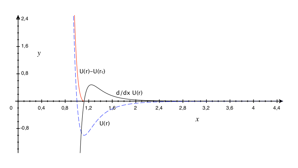
In practice, the L-J potential is cutoff beyond a specified distance $r_{c}$ and the potential at the cutoff distance is zero.

Figure 1: Lennard-Jones potential

Units

Novice users must understand that ESPResSo has no fixed unit system. The unit system is set by the user. Conventionally, reduced units are employed, in other words LJ units.

First steps

What is ESPResSo? It is an extensible, efficient Molecular Dynamics package specially powerful on simulating charged systems. In depth information about the package can be found in the relevant sources [1,4,2,3].

ESPResSo consists of two components. The simulation engine is written in C++ for the sake of computational efficiency. The steering or control level is interfaced to the kernel via an interpreter of the Python scripting languages.

The kernel performs all computationally demanding tasks. Before all, integration of Newton's equations of motion, including calculation of energies and forces. It also takes care of internal organization of data, storing the data about particles, communication between different processors or cells of the cell-system.

The scripting interface (Python) is used to setup the system (particles, boundary conditions, interactions etc.), control the simulation, run analysis, and store and load results. The user has at hand the full reliability and functionality of the scripting language. For instance, it is possible to use the SciPy package for analysis and PyPlot for plotting. With a certain overhead in efficiency, it can also be bused to reject/accept new configurations in combined MD/MC schemes. In principle, any parameter which is accessible from the scripting level can be changed at any moment of runtime. In this way methods like thermodynamic integration become readily accessible.

Note: This tutorial assumes that you already have a working ESPResSo installation on your system. If this is not the case, please consult the first chapters of the user's guide for installation instructions.

Python simulation scripts can be run conveniently:

import espressomd
print(espressomd.features())
required_features = ["LENNARD_JONES"]
espressomd.assert_features(required_features)

['ADDITIONAL_CHECKS', 'AFFINITY', 'BMHTF_NACL', 'BOND_CONSTRAINT', 'BUCKINGHAM', 'COLLISION_DETECTION', 'CUDA', 'DIPOLAR_BARNES_HUT', 'DIPOLAR_DIRECT_SUM', 'DIPOLES', 'DP3M', 'DPD', 'EK_BOUNDARIES', 'ELECTROKINETICS', 'ELECTROSTATICS', 'ENGINE', 'EXCLUSIONS', 'EXPERIMENTAL_FEATURES', 'EXTERNAL_FORCES', 'FFTW', 'GAUSSIAN', 'GAY_BERNE', 'GSL', 'H5MD', 'HAT', 'HERTZIAN', 'LANGEVIN_PER_PARTICLE', 'LB_BOUNDARIES', 'LB_BOUNDARIES_GPU', 'LB_ELECTROHYDRODYNAMICS', 'LENNARD_JONES', 'LENNARD_JONES_GENERIC', 'LJCOS', 'LJCOS2', 'LJGEN_SOFTCORE', 'MASS', 'MEMBRANE_COLLISION', 'METADYNAMICS', 'MMM1D_GPU', 'MORSE', 'NPT', 'P3M', 'PARTICLE_ANISOTROPY', 'ROTATION', 'ROTATIONAL_INERTIA', 'SMOOTH_STEP', 'SOFT_SPHERE', 'TABULATED', 'THOLE', 'VIRTUAL_SITES', 'VIRTUAL_SITES_INERTIALESS_TRACERS', 'VIRTUAL_SITES_RELATIVE', 'WCA']

Overview of a simulation script

Typically, a simulation script consists of the following parts:

• System setup (box geometry, thermodynamic ensemble, integrator parameters)
• Placing the particles
• Setup of interactions between particles
• Warm up (bringing the system into a state suitable for measurements)
• Integration loop (propagate the system in time and record measurements)

System setup

The functionality of ESPResSo for python is provided via a python module called espressomd. At the beginning of the simulation script, it has to be imported.

# Importing other relevant python modules
import numpy as np
# System parameters
N_PART = 100
DENSITY = 0.5

BOX_L = np.power(N_PART / DENSITY, 1.0 / 3.0) * np.ones(3)

The next step would be to create an instance of the System class and to seed espresso. This instance is used as a handle to the simulation system. At any time, only one instance of the System class can exist.

system = espressomd.System(box_l=BOX_L)
system.seed = 42

It can be used to manipulate the crucial system parameters like the time step and the size of the simulation box (time_step, and box_l).

SKIN = 0.4
TIME_STEP = 0.01

TEMPERATURE = 0.728
GAMMA=1.0

system.time_step = TIME_STEP
system.cell_system.skin = SKIN

Choosing the thermodynamic ensemble, thermostat

Simulations can be carried out in different thermodynamic ensembles such as NVE (particle Number, Volume, Energy), NVT (particle Number, Volume, Temperature) or NPT-isotropic (particle Number, Pressure, Temperature).

The NVE ensemble is simulated without a thermostat. A previously enabled thermostat can be switched off as follows:

system.thermostat.turn_off()

True

The NVT and NPT ensembles require a thermostat. In this tutorial, we use the Langevin thermostat.

In ESPResSo, the thermostat is set as follows:

system.thermostat.set_langevin(kT=TEMPERATURE, gamma=GAMMA, seed=42)

Use a Langevin thermostat (NVT or NPT ensemble) with temperature set to temperature and damping coefficient to GAMMA.

Placing and accessing particles

Particles in the simulation can be added and accessed via the part property of the System class. Individual particles are referred to by an integer id, e.g., system.part[0]. If id is unspecified, an unused particle id is automatically assigned. It is also possible to use common python iterators and slicing operations to add or access several particles at once.

Particles can be grouped into several types, so that, e.g., a binary fluid can be simulated. Particle types are identified by integer ids, which are set via the particles' type attribute. If it is not specified, zero is implied.

# Add particles to the simulation box at random positions
for i in range(N_PART):
    system.part.add(type=0, pos=np.random.random(3) * system.box_l)

# Access position of a single particle
print("position of particle with id 0:", system.part[0].pos)

# Iterate over the first five particles for the purpose of demonstration.
# For accessing all particles, use a slice: system.part[:]
for i in range(5):
    print("id", i, "position:", system.part[i].pos)
    print("id", i, "velocity:", system.part[i].v)

# Obtain all particle positions
cur_pos = system.part[:].pos

position of particle with id 0: [2.11957344 5.25116394 4.92709856]
id 0 position: [2.11957344 5.25116394 4.92709856]
id 0 velocity: [0. 0. 0.]
id 1 position: [5.79502016 4.8871939  0.44490466]
id 1 velocity: [0. 0. 0.]
id 2 position: [1.08409646 4.19129647 2.8459586 ]
id 2 velocity: [0. 0. 0.]
id 3 position: [3.55515501 2.54077072 2.65501185]
id 3 velocity: [0. 0. 0.]
id 4 position: [4.79870704 2.96108691 3.99776116]
id 4 velocity: [0. 0. 0.]

Many objects in ESPResSo have a string representation, and thus can be displayed via python's print function:

print(system.part[0])

ParticleHandle([('id', 0), ('pos', (2.119573440128747, 5.251163937147461, 4.927098561793697)), ('_id', 0), ('bond_site', (-1.0, -1.0, -1.0)), ('bonds', ()), ('dip', (0.0, 0.0, 0.0)), ('dipm', 0.0), ('director', (0.0, 0.0, 1.0)), ('exclusions', ()), ('ext_force', (0.0, 0.0, 0.0)), ('ext_torque', (0.0, 0.0, 0.0)), ('f', (0.0, 0.0, 0.0)), ('fix', (0, 0, 0)), ('gamma', (-1.0, -1.0, -1.0)), ('gamma_rot', (-1.0, -1.0, -1.0)), ('image_box', (0, 0, 0)), ('mass', 1.0), ('mol_id', 0), ('mu_E', (0.0, 0.0, 0.0)), ('node', 0), ('omega_body', (0.0, 0.0, 0.0)), ('omega_lab', (0.0, 0.0, 0.0)), ('out_direction', array([0., 0., 0.])), ('q', 0.0), ('quat', (1.0, 0.0, 0.0, 0.0)), ('rinertia', (1.0, 1.0, 1.0)), ('rotation', (0, 0, 0)), ('swimming', {'v_swim': 0.0, 'f_swim': 0.0, 'mode': 'N/A', 'dipole_length': 0.0}), ('temp', -1.0), ('torque_lab', (0.0, 0.0, 0.0)), ('type', 0), ('v', (0.0, 0.0, 0.0)), ('virtual', False), ('vs_quat', array([0., 0., 0., 0.])), ('vs_relative', (0, 0.0, array([0., 0., 0., 0.])))])

Setting up non-bonded interactions

Non-bonded interactions act between all particles of a given combination of particle types. In this tutorial, we use the Lennard-Jones non-bonded interaction. The interaction of two particles of type 0 can be setup as follows:

LJ_EPS = 1.0
LJ_SIG = 1.0
LJ_CUT = 2.5 * LJ_SIG
LJ_CAP = 0.5
system.non_bonded_inter[0, 0].lennard_jones.set_params(
    epsilon=LJ_EPS, sigma=LJ_SIG, cutoff=LJ_CUT, shift='auto')
system.force_cap = LJ_CAP

Warmup

In many cases, including this tutorial, particles are initially placed randomly in the simulation box. It is therefore possible that particles overlap, resulting in a huge repulsive force between them. In this case, integrating the equations of motion would not be numerically stable. Hence, it is necessary to remove this overlap. This is done by limiting the maximum force between two particles, integrating the equations of motion, and increasing the force limit step by step as follows:

WARM_STEPS = 100
WARM_N_TIME = 2000
MIN_DIST = 0.87

i = 0
act_min_dist = system.analysis.min_dist()
while i < WARM_N_TIME and act_min_dist < MIN_DIST:
    system.integrator.run(WARM_STEPS)
    act_min_dist = system.analysis.min_dist()
    i += 1
    LJ_CAP += 1.0
    system.force_cap = LJ_CAP

Integrating equations of motion and taking measurements

Once warmup is done, the force capping is switched off by setting it to zero.

system.force_cap = 0

At this point, we have set the necessary environment and warmed up our system. Now, we integrate the equations of motion and take measurements. We first plot the radial distribution function which describes how the density varies as a function of distance from a tagged particle. The radial distribution function is averaged over several measurements to reduce noise.

The potential and kinetic energies can be monitored using the analysis method system.analysis.energy(). Here kinetic_temperature refers to the measured temperature obtained from kinetic energy and the number of degrees of freedom in the system. It should fluctuate around the preset temperature of the thermostat.

The mean square displacement of particle $i$ is given by:

\begin{equation} \mathrm{msd}_i(t) =\langle (\vec{x}_i(t_0+t) -\vec{x}_i(t_0))^2\rangle, \end{equation}

and can be calculated using "observables and correlators". An observable is an object which takes a measurement on the system. It can depend on parameters specified when the observable is instanced, such as the ids of the particles to be considered.

# Integration parameters
sampling_interval = 100
sampling_iterations = 4000

from espressomd.observables import ParticlePositions
from espressomd.accumulators import Correlator
# Pass the ids of the particles to be tracked to the observable.
part_pos = ParticlePositions(ids=range(N_PART))
# Initialize MSD correlator
msd_corr = Correlator(obs1=part_pos,
                      tau_lin=10, delta_N=10,
                      tau_max=1000 * TIME_STEP,
                      corr_operation="square_distance_componentwise")
# Calculate results automatically during the integration
system.auto_update_accumulators.add(msd_corr)

# Set parameters for the radial distribution function
r_bins = 70
r_min = 0.0
r_max = system.box_l[0] / 2.0

avg_rdf = np.zeros((r_bins,))

# Take measurements
time = np.zeros(sampling_iterations)
instantaneous_temperature = np.zeros(sampling_iterations)
etotal = np.zeros(sampling_iterations)

for i in range(1, sampling_iterations + 1):
    system.integrator.run(sampling_interval)
    # Measure radial distribution function
    r, rdf = system.analysis.rdf(rdf_type="rdf", type_list_a=[0], type_list_b=[0],
                                 r_min=r_min, r_max=r_max, r_bins=r_bins)
    avg_rdf += rdf / sampling_iterations

    # Measure energies
    energies = system.analysis.energy()
    kinetic_temperature = energies['kinetic'] / (1.5 * N_PART)
    etotal[i - 1] = energies['total']
    time[i - 1] = system.time
    instantaneous_temperature[i - 1] = kinetic_temperature

# Finalize the correlator and obtain the results
msd_corr.finalize()
msd = msd_corr.result()

We now use the plotting library matplotlib available in Python to visualize the measurements.

import matplotlib.pyplot as plt
plt.ion()

fig1 = plt.figure(num=None, figsize=(10, 6), dpi=80, facecolor='w', edgecolor='k')
fig1.set_tight_layout(False)
plt.plot(r, avg_rdf, '-', color="#A60628", linewidth=2, alpha=1)
plt.xlabel('r $[\sigma]$', fontsize=20)
plt.ylabel('$g(r)$', fontsize=20)
plt.show()

fig2 = plt.figure(num=None, figsize=(10, 6), dpi=80, facecolor='w', edgecolor='k')
fig2.set_tight_layout(False)
plt.plot(time, instantaneous_temperature, '-', color="red", linewidth=2,
         alpha=0.5, label='Instantaneous Temperature')
plt.plot([min(time), max(time)], [TEMPERATURE] * 2, '-', color="#348ABD",
         linewidth=2, alpha=1, label='Set Temperature')
plt.xlabel(r'Time [$\delta t$]', fontsize=20)
plt.ylabel(r'$k_B$ Temperature [$k_B T$]', fontsize=20)
plt.legend(fontsize=16, loc=0)
plt.show()

Since the ensemble average $\langle E_\text{kin}\rangle=3/2 N k_B T$ is related to the temperature, we may compute the actual temperature of the system via $k_B T= 2/(3N) \langle E_\text{kin}\rangle$. The temperature is fixed and does not fluctuate in the NVT ensemble! The instantaneous temperature is calculated via $2/(3N) E_\text{kin}$ (without ensemble averaging), but it is not the temperature of the system.

The correlator output is stored in the array msd and has the following shape:

print(msd.shape)

(31, 302)

The first column of this array contains the lag time in units of the time step. The second column contains the number of values used to perform the averaging of the correlation. The next three columns contain the x, y and z mean squared displacement of the msd of the first particle. The next three columns then contain the x, y, z mean squared displacement of the next particle...

fig3 = plt.figure(num=None, figsize=(10, 6), dpi=80, facecolor='w', edgecolor='k')
fig3.set_tight_layout(False)
lag_time = msd[:, 0]
for i in range(0, N_PART, 30):
    msd_particle_i = msd[:, 2+i*3] + msd[:, 3+i*3] + msd[:, 4+i*3]
    plt.plot(lag_time, msd_particle_i,
             'o-', linewidth=2, label="particle id =" + str(i))
plt.xlabel(r'Lag time $\tau$ [$\delta t$]', fontsize=20)
plt.ylabel(r'Mean squared displacement [$\sigma^2$]', fontsize=20)
plt.xscale('log')
plt.yscale('log')
plt.legend()
plt.show()

Simple Error Estimation on Time Series Data

A simple way to estimate the error of an observable is to use the standard error of the mean (SE) for $N$ uncorrelated samples:

\begin{equation} SE = \sqrt{\frac{\sigma^2}{N}}, \end{equation}

where $\sigma^2$ is the variance

\begin{equation} \sigma^2 = \left\langle x^2 - \langle x\rangle^2 \right\rangle \end{equation}

# calculate the standard error of the mean of the total energy, assuming uncorrelatedness
standard_error_total_energy = np.sqrt(etotal.var()) / np.sqrt(sampling_iterations)
print(standard_error_total_energy)

0.2328724631583865

Exercises

Binary Lennard-Jones Liquid

A two-component Lennard-Jones liquid can be simulated by placing particles of two types (0 and 1) into the system. Depending on the Lennard-Jones parameters, the two components either mix or separate.

1. Modify the code such that half of the particles are of type=1. Type 0 is implied for the remaining particles.
2. Specify Lennard-Jones interactions between type 0 particles with other type 0 particles, type 1 particles with other type 1 particles, and type 0 particles with type 1 particles (set parameters for system.non_bonded_inter[i,j].lennard_jones where {i,j} can be {0,0}, {1,1}, and {0,1}. Use the same Lennard-Jones parameters for interactions within a component, but use a different lj_cut_mixed parameter for the cutoff of the Lennard-Jones interaction between particles of type 0 and particles of type 1. Set this parameter to $2^{\frac16}\sigma$ to get de-mixing or to $2.5\sigma$ to get mixing between the two components.
3. Record the radial distribution functions separately for particles of type 0 around particles of type 0, type 1 around particles of type 1, and type 0 around particles of type 1. This can be done by changing the type_list arguments of the system.analysis.rdf() command. You can record all three radial distribution functions in a single simulation. It is also possible to write them as several columns into a single file.
4. Plot the radial distribution functions for all three combinations of particle types. The mixed case will differ significantly, depending on your choice of lj_cut_mixed. Explain these differences.

References

[1] http://espressomd.org
[2] HJ Limbach, A. Arnold, and B. Mann. ESPResSo; an extensible simulation package for research on soft matter systems. Computer Physics Communications, 174(9):704–727, 2006.
[3] A. Arnold, O. Lenz, S. Kesselheim, R. Weeber, F. Fahrenberger, D. Rohm, P. Kosovan, and C. Holm. ESPResSo 3.1 — molecular dynamics software for coarse-grained models. In M. Griebel and M. A. Schweitzer, editors, Meshfree Methods for Partial Differential Equations VI, volume 89 of Lecture Notes in Computational Science and Engineering, pages 1–23. Springer Berlin Heidelberg, 2013.
[4] A. Arnold, BA Mann, HJ Limbach, and C. Holm. ESPResSo–An Extensible Simulation Package for Research on Soft Matter Systems. Forschung und wissenschaftliches Rechnen, 63:43–59, 2003.