This tutorial introduces some of the basic features of ESPResSo for charged systems by constructing a simulation script for a simple salt crystal. In the subsequent task, we use a more realistic force-field for a NaCl crystal. Finally, we introduce constraints and 2D-Electrostatics to simulate a molten salt in a parallel plate capacitor. We assume that the reader is familiar with the basic concepts of Python and MD simulations. Compile ESPResSo with the following features in your myconfig.hpp to be set throughout the whole tutorial:
#define EXTERNAL_FORCES
#define MASS
#define ELECTROSTATICS
#define WCA
The script for the tutorial can be found in your build directory at /doc/tutorials/02-charged_system/scripts/nacl.py. We start by importing numpy, pyplot, espressomd and setting up the simulation parameters:
from espressomd import System, electrostatics
import espressomd
import numpy
import matplotlib.pyplot as plt
plt.ion()

# Print enabled features
required_features = ["EXTERNAL_FORCES", "MASS", "ELECTROSTATICS", "WCA"]
espressomd.assert_features(required_features)
print(espressomd.features())

# System Parameters
n_part = 200
n_ionpairs = n_part / 2
density = 0.5
time_step = 0.01
temp = 1.0
gamma = 1.0
l_bjerrum = 7.0

num_steps_equilibration = 200
num_configs = 100
integ_steps_per_config = 250

# Particle Parameters
types       = {"Anion":          0, "Cation": 1}
numbers     = {"Anion": n_ionpairs, "Cation": n_ionpairs}
charges     = {"Anion":       -1.0, "Cation": 1.0}
wca_sigmas   = {"Anion":        1.0, "Cation": 1.0}
wca_epsilons = {"Anion":        1.0, "Cation": 1.0}
['ADDITIONAL_CHECKS', 'AFFINITY', 'BMHTF_NACL', 'BOND_CONSTRAINT', 'BUCKINGHAM', 'COLLISION_DETECTION', 'CUDA', 'DIPOLAR_BARNES_HUT', 'DIPOLAR_DIRECT_SUM', 'DIPOLES', 'DP3M', 'DPD', 'EK_BOUNDARIES', 'ELECTROKINETICS', 'ELECTROSTATICS', 'ENGINE', 'EXCLUSIONS', 'EXPERIMENTAL_FEATURES', 'EXTERNAL_FORCES', 'FFTW', 'GAUSSIAN', 'GAY_BERNE', 'GSL', 'H5MD', 'HAT', 'HERTZIAN', 'LANGEVIN_PER_PARTICLE', 'LB_BOUNDARIES', 'LB_BOUNDARIES_GPU', 'LB_ELECTROHYDRODYNAMICS', 'LENNARD_JONES', 'LENNARD_JONES_GENERIC', 'LJCOS', 'LJCOS2', 'LJGEN_SOFTCORE', 'MASS', 'MEMBRANE_COLLISION', 'METADYNAMICS', 'MMM1D_GPU', 'MORSE', 'NPT', 'P3M', 'PARTICLE_ANISOTROPY', 'ROTATION', 'ROTATIONAL_INERTIA', 'SMOOTH_STEP', 'SOFT_SPHERE', 'TABULATED', 'THOLE', 'VIRTUAL_SITES', 'VIRTUAL_SITES_INERTIALESS_TRACERS', 'VIRTUAL_SITES_RELATIVE', 'WCA']
These variables do not change anything in the simulation engine, but are just standard Python variables. They are used to increase the readability and flexibility of the script. The box length is not a parameter of this simulation, it is calculated from the number of particles and the system density. This allows to change the parameters later easily, e.g. to simulate a bigger system. We use dictionaries for all particle related parameters, which is less error-prone and readable as we will see later when we actually need the values. The parameters here define a purely repulsive, equally sized, monovalent salt.
The simulation engine itself is modified by changing the espressomd.System() properties. We create an instance system and set the box length, periodicity and time step. The skin depth skin is a parameter for the link--cell system which tunes its performance, but shall not be discussed here.
# Setup System
box_l = (n_part / density)**(1. / 3.)
system = System(box_l=[box_l, box_l, box_l])
system.seed = 42
system.periodicity = [True, True, True]
system.time_step = time_step
system.cell_system.skin = 0.3
We now fill this simulation box with particles at random positions, using type and charge from our dictionaries. Using the length of the particle list system.part for the id, we make sure that our particles are numbered consecutively. The particle type is used to link non-bonded interactions to a certain group of particles.
for i in range(int(n_ionpairs)):
    system.part.add(id=len(system.part), type=types["Anion"],
                    pos=numpy.random.random(3) * box_l, q=charges["Anion"])
for i in range(int(n_ionpairs)):
    system.part.add(id=len(system.part), type=types["Cation"],
                    pos=numpy.random.random(3) * box_l, q=charges["Cation"])
Before we can really start the simulation, we have to specify the interactions between our particles. We already defined the WCA parameters at the beginning, what is left is to specify the combination rule and to iterate over particle type pairs. For simplicity, we implement only the Lorentz-Berthelot rules. We pass our interaction pair to system.non_bonded_inter[\*,\*] and set the pre-calculated WCA parameters epsilon and sigma.
def combination_rule_epsilon(rule, eps1, eps2):
    if rule == "Lorentz":
        return (eps1 * eps2)**0.5
    else:
        return ValueError("No combination rule defined")

def combination_rule_sigma(rule, sig1, sig2):
    if rule == "Berthelot":
        return (sig1 + sig2) * 0.5
    else:
        return ValueError("No combination rule defined")

# WCA interactions parameters
for s in [["Anion", "Cation"], ["Anion", "Anion"], ["Cation", "Cation"]]:
    wca_sig = combination_rule_sigma("Berthelot", wca_sigmas[s[0]], wca_sigmas[s[1]])
    wca_eps = combination_rule_epsilon("Lorentz", wca_epsilons[s[0]], wca_epsilons[s[1]])

    system.non_bonded_inter[types[s[0]], types[s[1]]].wca.set_params(
        epsilon=wca_eps, sigma=wca_sig)
With randomly positioned particles, we most likely have huge overlap and the strong repulsion will cause the simulation to crash. The next step in our script therefore is a suitable WCA equilibration. This is known to be a tricky part of a simulation and several approaches exist to reduce the particle overlap. Here, we use the steepest descent algorithm and cap the maximal particle displacement per integration step to 1% of sigma. We use system.analysis.min_dist() to get the minimal distance between all particles pairs. This value is used to stop the minimization when particles are far away enough from each other. At the end, we activate the Langevin thermostat for our NVT ensemble with temperature temp and friction coefficient gamma.
# WCA Equilibration
max_sigma = max(wca_sigmas.values())
min_dist = 0.0
system.minimize_energy.init(f_max=0, gamma=10.0, max_steps=10,
                            max_displacement=max_sigma * 0.01)

while min_dist < max_sigma:
    min_dist = system.analysis.min_dist([types["Anion"], types["Cation"]],
                                        [types["Anion"], types["Cation"]])
    system.minimize_energy.minimize()

# Set thermostat
system.thermostat.set_langevin(kT=temp, gamma=gamma, seed=42)
ESPResSo uses so-called actors for electrostatics, magnetostatics and hydrodynamics. This ensures that unphysical combinations of algorithms are avoided, for example simultaneous usage of two electrostatic interactions. Adding an actor to the system also activates the method and calls necessary initialization routines. Here, we define a P$^3$M object with parameters Bjerrum length and rms force error. This automatically starts a tuning function which tries to find optimal parameters for P$^3$M and prints them to the screen:
p3m = electrostatics.P3M(prefactor=l_bjerrum * temp,
                         accuracy=1e-3)
system.actors.add(p3m)
P3M tune parameters: Accuracy goal = 1.00000e-03 prefactor = 7.00000e+00
System: box_l = 7.36806e+00 # charged part = 200 Sum[q_i^2] = 2.00000e+02
mesh cao r_cut_iL     alpha_L      err          rs_err     ks_err     time [ms]
6    7   cao too large for this mesh
8    7   4.59284e-01 6.50911e+00 8.77128e-02 7.071e-04 8.771e-02 accuracy not achieved
8    7   4.59284e-01 6.50911e+00 8.77128e-02 7.071e-04 8.771e-02 accuracy not achieved
8    7   4.59284e-01 6.50911e+00 8.77128e-02 7.071e-04 8.771e-02 accuracy not achieved
10   7   4.59284e-01 6.50911e+00 1.39625e-02 7.071e-04 1.394e-02 accuracy not achieved
10   7   4.59284e-01 6.50911e+00 1.39625e-02 7.071e-04 1.394e-02 accuracy not achieved
10   7   4.59284e-01 6.50911e+00 1.39625e-02 7.071e-04 1.394e-02 accuracy not achieved
12   7   4.59284e-01 6.50911e+00 2.51196e-03 7.071e-04 2.410e-03 accuracy not achieved
12   7   4.59284e-01 6.50911e+00 2.51196e-03 7.071e-04 2.410e-03 accuracy not achieved
12   7   4.59284e-01 6.50911e+00 2.51196e-03 7.071e-04 2.410e-03 accuracy not achieved
14   7   4.44034e-01 6.73901e+00 9.96813e-04 7.071e-04 7.026e-04 1.24
14   6   4.59284e-01 6.50911e+00 1.30343e-03 7.071e-04 1.095e-03 accuracy not achieved
14   7   4.44034e-01 6.73901e+00 9.96813e-04 7.071e-04 7.026e-04 1.25
14   6   4.44034e-01 6.73901e+00 1.65807e-03 7.071e-04 1.500e-03 accuracy not achieved
16   7   3.92866e-01 7.64271e+00 9.88469e-04 7.071e-04 6.907e-04 1.04
16   6   4.26689e-01 7.02075e+00 9.95097e-04 7.071e-04 7.002e-04 0.96
16   5   4.44034e-01 6.73901e+00 1.71326e-03 7.071e-04 1.561e-03 accuracy not achieved
16   6   4.26689e-01 7.02075e+00 9.95097e-04 7.071e-04 7.002e-04 0.96
16   5   4.26689e-01 7.02075e+00 2.19825e-03 7.071e-04 2.081e-03 accuracy not achieved
16   7   3.92521e-01 7.64963e+00 9.93284e-04 7.071e-04 6.976e-04 1.04
16   6   4.26689e-01 7.02075e+00 9.95097e-04 7.071e-04 7.002e-04 0.96
16   5   4.26689e-01 7.02075e+00 2.19825e-03 7.071e-04 2.081e-03 accuracy not achieved
16   7   3.92521e-01 7.64963e+00 9.93284e-04 7.071e-04 6.976e-04 1.03
18   6   3.83353e-01 7.83768e+00 9.90888e-04 7.071e-04 6.942e-04 1.47
18   5   4.26689e-01 7.02075e+00 1.20437e-03 7.071e-04 9.749e-04 accuracy not achieved
18   7   3.51685e-01 8.56382e+00 9.96029e-04 7.071e-04 7.015e-04 1.57
18   6   3.82605e-01 7.85345e+00 9.99544e-04 7.071e-04 7.065e-04 1.17
18   5   3.83353e-01 7.83768e+00 2.20682e-03 7.071e-04 2.090e-03 accuracy not achieved
18   7   3.51906e-01 8.55828e+00 9.92553e-04 7.071e-04 6.965e-04 1.24
18   6   3.82605e-01 7.85345e+00 9.99544e-04 7.071e-04 7.065e-04 1.17
18   5   3.82605e-01 7.85345e+00 2.23516e-03 7.071e-04 2.120e-03 accuracy not achieved
18   7   3.51966e-01 8.55679e+00 9.91618e-04 7.071e-04 6.952e-04 1.25
20   6   3.47483e-01 8.67026e+00 9.97735e-04 7.071e-04 7.039e-04 1.41
20   5   3.82605e-01 7.85345e+00 1.28733e-03 7.071e-04 1.076e-03 accuracy not achieved
20   7   3.19086e-01 9.46400e+00 9.92894e-04 7.071e-04 6.970e-04 1.39
20   6   3.19086e-01 9.46400e+00 1.68949e-03 7.071e-04 1.534e-03 accuracy not achieved
20   7   3.19086e-01 9.46400e+00 9.92894e-04 7.071e-04 6.970e-04 1.22
20   6   3.19086e-01 9.46400e+00 1.68949e-03 7.071e-04 1.534e-03 accuracy not achieved
22   6   3.18463e-01 9.48302e+00 9.96788e-04 7.071e-04 7.026e-04 1.49
22   5   3.19086e-01 9.46400e+00 2.23654e-03 7.071e-04 2.122e-03 accuracy not achieved
22   7   2.92288e-01 1.03565e+01 9.88585e-04 7.071e-04 6.909e-04 1.35
22   6   2.92288e-01 1.03565e+01 1.69049e-03 7.071e-04 1.535e-03 accuracy not achieved
22   7   2.91717e-01 1.03773e+01 9.99339e-04 7.071e-04 7.062e-04 1.34
22   6   2.92288e-01 1.03565e+01 1.69049e-03 7.071e-04 1.535e-03 accuracy not achieved
22   6   2.91717e-01 1.03773e+01 1.71612e-03 7.071e-04 1.564e-03 accuracy not achieved
22   7   2.91717e-01 1.03773e+01 9.99339e-04 7.071e-04 7.062e-04 1.35
22   6   2.91717e-01 1.03773e+01 1.71612e-03 7.071e-04 1.564e-03 accuracy not achieved
24   6   2.91717e-01 1.03773e+01 1.03369e-03 7.071e-04 7.540e-04 accuracy not achieved
24   7   2.69497e-01 1.12572e+01 9.90604e-04 7.071e-04 6.938e-04 1.48
24   6   2.91717e-01 1.03773e+01 1.03369e-03 7.071e-04 7.540e-04 accuracy not achieved
24   6   2.69497e-01 1.12572e+01 1.70571e-03 7.071e-04 1.552e-03 accuracy not achieved
24   7   2.69497e-01 1.12572e+01 9.90604e-04 7.071e-04 6.938e-04 1.48
24   6   2.69497e-01 1.12572e+01 1.70571e-03 7.071e-04 1.552e-03 accuracy not achieved
24   6   2.69497e-01 1.12572e+01 1.70571e-03 7.071e-04 1.552e-03 accuracy not achieved
24   7   2.69497e-01 1.12572e+01 9.90604e-04 7.071e-04 6.938e-04 1.73
24   6   2.69497e-01 1.12572e+01 1.70571e-03 7.071e-04 1.552e-03 accuracy not achieved
26   6   2.69497e-01 1.12572e+01 1.06326e-03 7.071e-04 7.941e-04 accuracy not achieved
26   7   2.50021e-01 1.21588e+01 9.94234e-04 7.071e-04 6.989e-04 1.97
26   6   2.69497e-01 1.12572e+01 1.06326e-03 7.071e-04 7.941e-04 accuracy not achieved
26   6   2.50021e-01 1.21588e+01 1.72416e-03 7.071e-04 1.572e-03 accuracy not achieved
26   7   2.50021e-01 1.21588e+01 9.94234e-04 7.071e-04 6.989e-04 1.97
26   6   2.50021e-01 1.21588e+01 1.72416e-03 7.071e-04 1.572e-03 accuracy not achieved
26   6   2.50021e-01 1.21588e+01 1.72416e-03 7.071e-04 1.572e-03 accuracy not achieved
26   7   2.50021e-01 1.21588e+01 9.94234e-04 7.071e-04 6.989e-04 1.95
26   6   2.50021e-01 1.21588e+01 1.72416e-03 7.071e-04 1.572e-03 accuracy not achieved
28   6   2.50021e-01 1.21588e+01 1.10215e-03 7.071e-04 8.454e-04 accuracy not achieved
28   7   2.33418e-01 1.30478e+01 9.93562e-04 7.071e-04 6.980e-04 2.37
28   6   2.50021e-01 1.21588e+01 1.10215e-03 7.071e-04 8.454e-04 accuracy not achieved
28   6   2.33418e-01 1.30478e+01 1.73159e-03 7.071e-04 1.581e-03 accuracy not achieved
28   7   2.33418e-01 1.30478e+01 9.93562e-04 7.071e-04 6.980e-04 2.37
28   6   2.33418e-01 1.30478e+01 1.73159e-03 7.071e-04 1.581e-03 accuracy not achieved
30   6   2.33418e-01 1.30478e+01 1.13441e-03 7.071e-04 8.871e-04 accuracy not achieved
30   7   2.18830e-01 1.39419e+01 9.96010e-04 7.071e-04 7.015e-04 2.75
30   6   2.33418e-01 1.30478e+01 1.13441e-03 7.071e-04 8.871e-04 accuracy not achieved
30   6   2.18830e-01 1.39419e+01 1.74605e-03 7.071e-04 1.596e-03 accuracy not achieved
30   7   2.18830e-01 1.39419e+01 9.96010e-04 7.071e-04 7.015e-04 2.74
30   6   2.18830e-01 1.39419e+01 1.74605e-03 7.071e-04 1.596e-03 accuracy not achieved
30   6   2.18830e-01 1.39419e+01 1.74605e-03 7.071e-04 1.596e-03 accuracy not achieved
30   7   2.18830e-01 1.39419e+01 9.96010e-04 7.071e-04 7.015e-04 2.73
30   6   2.18830e-01 1.39419e+01 1.74605e-03 7.071e-04 1.596e-03 accuracy not achieved
32   6   2.18830e-01 1.39419e+01 1.16848e-03 7.071e-04 9.302e-04 accuracy not achieved
32   7   2.06008e-01 1.48336e+01 9.98377e-04 7.071e-04 7.048e-04 2.65
32   6   2.18830e-01 1.39419e+01 1.16848e-03 7.071e-04 9.302e-04 accuracy not achieved
32   6   2.06008e-01 1.48336e+01 1.75996e-03 7.071e-04 1.612e-03 accuracy not achieved
32   7   2.06008e-01 1.48336e+01 9.98377e-04 7.071e-04 7.048e-04 2.62
32   6   2.06008e-01 1.48336e+01 1.75996e-03 7.071e-04 1.612e-03 accuracy not achieved
32   6   2.06008e-01 1.48336e+01 1.75996e-03 7.071e-04 1.612e-03 accuracy not achieved
32   7   2.06008e-01 1.48336e+01 9.98377e-04 7.071e-04 7.048e-04 2.66
32   6   2.06008e-01 1.48336e+01 1.75996e-03 7.071e-04 1.612e-03 accuracy not achieved
34   6   2.06008e-01 1.48336e+01 1.20079e-03 7.071e-04 9.705e-04 accuracy not achieved
34   7   1.94741e-01 1.57154e+01 9.97945e-04 7.071e-04 7.042e-04 6.22
34   6   2.06008e-01 1.48336e+01 1.20079e-03 7.071e-04 9.705e-04 accuracy not achieved

resulting parameters: mesh: (16 16 16), cao: 6, r_cut_iL: 4.2669e-01,
                      alpha_L: 7.0208e+00, accuracy: 9.9510e-04, time: 0.96
Before the production part of the simulation, we do a quick temperature equilibration. For the output, we gather all energies with system.analysis.energy(), calculate the "current" temperature from the ideal part and print it to the screen along with the total and Coulomb energies. Note that for the ideal gas the temperature is given via $1/2 m \sqrt{\langle v^2 \rangle}=3/2 k_BT$, where $\langle \cdot \rangle$ denotes the ensemble average. Calculating some kind of "current temperature" via $T_\text{cur}=\frac{m}{3 k_B} \sqrt{ v^2 }$ won't produce the temperature in the system. Only when averaging the squared velocities first one would obtain the temperature for the ideal gas. $T$ is a fixed quantity and does not fluctuate in the canonical ensemble.
We integrate for a certain amount of steps with system.integrator.run(100).
# Temperature Equilibration
system.time = 0.0
for i in range(int(num_steps_equilibration / 50)):
    energy = system.analysis.energy()
    temp_measured = energy['kinetic'] / ((3.0 / 2.0) * n_part)
    print("t={0:.1f}, E_total={1:.2f}, E_coulomb={2:.2f},T={3:.4f}"
          .format(system.time, energy['total'], energy['coulomb'], temp_measured), end='\r')
    system.integrator.run(200)

print()
t=6.0, E_total=-474.20, E_coulomb=-855.08,T=0.9412
Now we can integrate the particle trajectories for a couple of time steps. Our integration loop basically looks like the equilibration:
# Integration
system.time = 0.0
for i in range(num_configs):
    energy = system.analysis.energy()
    temp_measured = energy['kinetic'] / ((3.0 / 2.0) * n_part)
    print("progress={:.0f}%, t={:.1f}, E_total={:.2f}, E_coulomb={:.2f}, T={:.4f}"
          .format((i + 1) * 100. / num_configs, system.time, energy['total'],
                  energy['coulomb'], temp_measured), end='\r')
    system.integrator.run(integ_steps_per_config)

    # Internally append particle configuration
    system.analysis.append()

print()
progress=100%, t=247.5, E_total=-494.84, E_coulomb=-866.97, T=0.9913
Additionally, we append all particle configurations in the core with system.analysis.append() for a very convenient analysis later on.
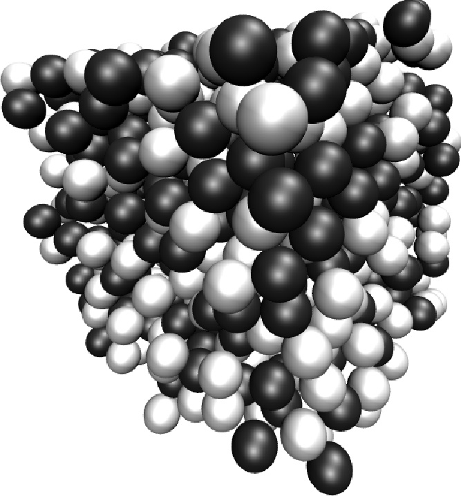
Now, we want to calculate the averaged radial distribution functions $g_{++}(r)$ and $g_{+-}(r)$ with the rdf() command from system.analysis:
# Analysis
# Calculate the averaged rdfs
rdf_bins = 100
r_min = 0.0
r_max = system.box_l[0] / 2.0
r, rdf_00 = system.analysis.rdf(rdf_type='<rdf>',
                                type_list_a=[types["Anion"]],
                                type_list_b=[types["Anion"]],
                                r_min=r_min,
                                r_max=r_max,
                                r_bins=rdf_bins)
r, rdf_01 = system.analysis.rdf(rdf_type='<rdf>',
                                type_list_a=[types["Anion"]],
                                type_list_b=[types["Cation"]],
                                r_min=r_min,
                                r_max=r_max,
                                r_bins=rdf_bins)
The shown rdf() commands return the radial distribution functions for equally and oppositely charged particles for specified radii and number of bins. In this case, we calculate the averaged rdf of the stored configurations, denoted by the chevrons in rdf_type='$<\mathrm{rdf}>$'. Using rdf_type='rdf' would simply calculate the rdf of the current particle configuration. The results are two NumPy arrays containing the $r$ and $g(r)$ values. We can then write the data into a file with standard python output routines.
with open('rdf.data', 'w') as rdf_fp:
    for i in range(rdf_bins):
        rdf_fp.write("%1.5e %1.5e %1.5e\n" % (r[i], rdf_00[i], rdf_01[i]))
Finally we can plot the two radial distribution functions using pyplot.
# Plot the distribution functions
plt.figure(figsize=(10, 6), dpi=80)
plt.plot(r[:], rdf_00[:], label='Na$-$Na')
plt.plot(r[:], rdf_01[:], label='Na$-$Cl')
plt.xlabel('$r$', fontsize=20)
plt.ylabel('$g(r)$', fontsize=20)
plt.legend(fontsize=20)
plt.show()

So far, the system has arbitrary units and is not connected to any real physical system. Simulate a proper NaCl crystal with the force field parameter taken from [1]:
| Ion | $q/\mathrm{e}$ | $\sigma/\mathrm{\mathring{A}}$ | $(\epsilon/\mathrm{k_B})/\mathrm{K}$ | $m/\mathrm{u}$ |
|---|---|---|---|---|
| Na | +1 | 2.52 | 17.44 | 22.99 |
| Cl | -1 | 3.85 | 192.45 | 35.453 |
Use the following system parameters:
| Parameter | Value |
|---|---|
| Temperature | $298\ \mathrm{K}$ |
| Fiction Coeff. | $ 10\ \mathrm{ps}^{-1}$ |
| Density | $1.5736\ \mathrm{u \mathring{A}}^{-3}$ |
| Bjerrum Length (298 K) | $439.2\ \mathrm{\mathring{A}}$ |
| Time Step | $2\ \mathrm{fs}$ |
To make your life easier, don't try to equilibrate randomly positioned particles, but set them up in a crystal structure close to equilibrium. If you do it right, you don't even need the WCA equilibration. To speed things up, don't go further than 1000 particles and use a P$^3$M accuracy of $10^{-2}$. Your RDF should look like the plot in figure 2. If you get stuck, you can look at the solution script /doc/tutorials/02-charged_system/scripts/nacl_units.py (or nacl_units_vis.py with visualization).
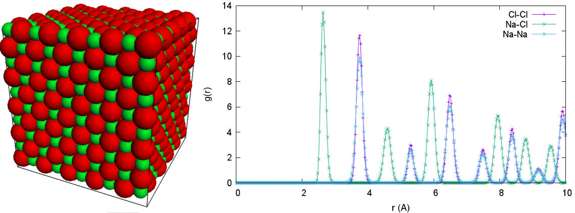
[1] R. Fuentes-Azcatl and M. Barbosa, Sodium Chloride, NaCl/$\epsilon$ : New Force Field, J. Phys. Chem. B, 2016, 120(9), pp 2460-2470.