Tutorial 4 : The lattice Boltzmann Method in ESPResSo - Part 1

Before you start:

With this tutorial you can get started using the lattice Boltzmann method for hydrodynamics. We give a brief introduction about the theory and how to use the method in ESPResSo. We have selected two interesting problems for which LB can be applied and which are well understood. You can start with any of them.

The tutorial is relatively long and working through it carefully is work for at least a full day. You can however get a glimpse of different aspects by starting to work on the tasks.

Note: LB cannot be used as a black box. It is unavoidable to spend time learning the theory and gaining practical experience.

1 Introduction

In this tutorial, you will learn the basics of the lattice Boltzmann Method (LBM) with special focus on the application on soft matter simulations or more precisely on how to apply it in combination with molecular dynamics to take into account hydrodynamic solvent effects without the need to introduce thousands of solvent particles.

The LBM – its theory as well as its applications – is still a very active field of research. After almost 20 years of development there are many cases in which the LBM has proven to be fruitful, in other cases the LBM is considered promising, and in some cases it has not been of any help. We encourage you to contribute to the scientific discussion of the LBM because there is still a lot that is unknown or only vaguely known about this fascinating method.

Tutorial Outline

This tutorial should enable you to start a scientific project applying the LB method with ESPResSo. In the first part we summarize a few basic ideas behind LB and describe the interface. In the second part we suggest three different classic examples where hydrodynamics are important. These are

Notes on the ESPResSo version you will need

ESPResSo offers both CPU and GPU support for LB. We recommend using the GPU code, as it is much (100x) faster than the CPU code.

For the tutorial you will have to compile in the following features:

2 The LBM in brief

Linearized Boltzmann equation

Here we want to repeat a few very basic facts about the LBM. You will find much better introductions in various books and articles, e.g. [1, 2]. It will however help clarifying our choice of words and we will eventually say something about the implementation in ESPResSo. It is very loosely written, with the goal that the reader understands basic concepts and how they are implemented in ESPResSo.

The LBM essentially consists of solving a fully discretized version of the linearized Boltzmann equation. The Boltzmann equation describes the time evolution of the one particle distribution function $f \left(\vec{x}, \vec{p}, t\right)$, which is the probability of finding a molecule in a phase space volume $d^3\vec{x}\,d^3\vec{p}$ at time $t$.The function $f$ is normalized so that the integral over the whole phase space is the total mass of the particles:

$$\int \int f \left(\vec{x}, \vec{p}, t\right) \,d^3\vec{x}\,d^3\vec{p} = N,$$

where $N$ denotes the particle number. The quantity $f\left(\vec{x}, \vec{p}, t\right) \,d^3\vec{x}\,d^3\vec{p}$ corresponds to the number of particles in this particular cell of the phase space, the population.

Discretization

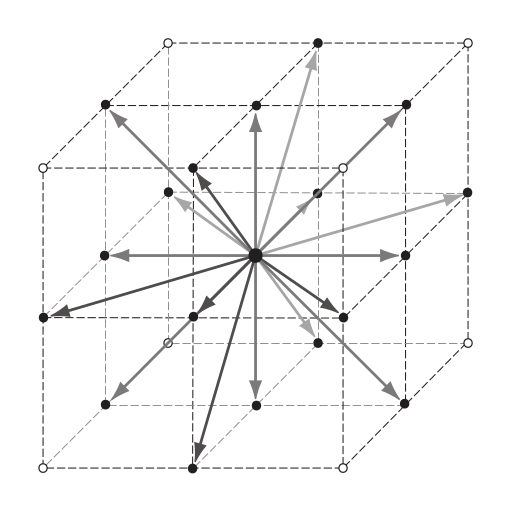
The LBM discretizes the Boltzmann equation not only in real space (the lattice!) and time, but also the velocity space is discretized. A surprisingly small number of velocities, usually 19 in 3D, is sufficient to describe incompressible, viscous flow correctly. Mostly we will refer to the three-dimensional model with a discrete set of 19 velocities, which is conventionally called D3Q19. These velocities, $\vec{c_i}$ , are chosen such that they correspond to the movement from one lattice node to another in one time step. A two step scheme is used to transport information through the system. In the streaming step the particles (in terms of populations) are transported to the cell where the corresponding velocity points to. In the collision step, the distribution functions in each cell are relaxed towards the local thermodynamic equilibrium. This will be described in more detail below.

The hydrodynamic fields, the density $\rho$, the fluid momentum density $\vec{j}$ and the pressure tensor $\Pi$ can be calculated straightforwardly from the populations. They correspond to the moments of the distribution function:

\begin{align} \rho &= \sum_i f_i \\ \vec{j} = \rho \vec{u} &= \sum_i f_i \vec{c_i} \\ \Pi^{\alpha \beta} &= \sum_i f_i \vec{c_i}^{\alpha}\vec{c_i}^{\beta} \label{eq:fields} \end{align}

Here the Greek indices denotes the cartesian axis and the Latin indices indicate the number in the discrete velocity set. Note that the pressure tensor is symmetric. It is easy to see that these equations are linear transformations of the $f_i$ and that they carry the most important information. They are 10 independent variables, but this is not enough to store the full information of 19 populations. Therefore 9 additional quantities are introduced. Together they form a different basis set of the 19-dimensional population space, the modes space and the modes are denoted by $m_i$. The 9 extra modes are referred to as kinetic modes or ghost modes. It is possible to explicitly write down the base transformation matrix, and its inverse and in the ESPResSo LBM implementation this basis transformation is made for every cell in every LBM step.

The 19 velocity vectors $\vec{c_i}$ for a D3Q19 lattice. From the central grid point, the velocity vectors point towards all 18 nearest neighbours marked by filled circles. The 19th velocity vector is the rest mode (zero velocity).

The second step: collision

The second step is the collision part, where the actual physics happens. For the LBM it is assumed that the collision process linearly relaxes the populations to the local equilibrium, thus that it is a linear (=matrix) operator acting on the populations in each LB cell. It should conserve the particle number and the momentum. At this point it is clear why the mode space is helpful. A 19 dimensional matrix that conserves the first 4 modes (with the eigenvalue 1) is diagonal in the first four rows and columns. By symmetry consideration one finds that only four independent variables are enough to characterize the linear relaxation process so that all symmetries of the lattice are obeyed. Two of them are closely related to the shear and bulk viscosity of the fluid, and two of them do not have a direct physical equivalent. They are just called relaxation rates of the kinetic modes.

In mode space the equilibrium distribution is calculated from the local density and velocity. The kinetic modes 11-19 have the value 0 at equilibrium. The collision operator is diagonal in mode space and has the form

\begin{align*} m^\star_i &= \gamma_i \left( m_i - m_i^\text{eq} \right) + m_i ^\text{eq}. \end{align*}

Here $m^\star_i$ is the $i$th mode after the collision. In other words: each mode is relaxed towards its equilibrium value with a relaxation rate $\gamma_i$. The conserved modes are not relaxed, i.e. their relaxation rate is 1.

By symmetry consideration one finds that only four independent relaxation rates are allowed. We summarize them here.

\begin{align*} m^\star_i &= \gamma_i m_i \\ \gamma_1=\dots=\gamma_4&=1 \\ \gamma_5&=\gamma_\text{b} \\ \gamma_6=\dots=\gamma_{10}&=\gamma_\text{s} \\ \gamma_{11}=\dots=\gamma_{16}&=\gamma_\text{odd} \\ \gamma_{17}=\dots = \gamma_{19}&=\gamma_\text{even} \\ \end{align*}

To include hydrodynamic fluctuations of the fluid, random fluctuations are added to the nonconserved modes $5\dots 19$ on every LB node so that the LB fluid temperature is well defined and the corresponding fluctuation formula holds, according to the fluctuation dissipation theorem. An extensive discussion of this topic is found in [3].

Particle coupling

In ESPResSo particles are coupled to the LB fluid via the so-called force coupling method: the fluid velocity $\vec{u}$ at the position of a particle is calculated via trilinear interpolation and a force is applied on the particle that is proportional to the velocity difference between particle and fluid:

\begin{equation} \vec{F}_H = - \gamma \left(\vec{v}-\vec{u}\right) \end{equation}

The opposite force is distributed on the surrounding LB nodes. Additionally a random force is added to maintain a constant temperature, according to the fluctuation dissipation theorem.

The coupling scheme between fluid and particles is based on the interpolation of the fluid velocity $\vec{u}$ from the grid nodes. This is done by trilinear interpolation. The difference between the particle velocity $\vec{v}(t)$ and the interpolated velocity $\vec{u}(\vec{r},t)$ is used in the momentum exchange of the equation $\vec{F}_H$ above.

3 The LB interface in ESPResSo

ESPResSo features two virtually independent implementations of LB. One implementation uses CPUs and one uses a GPU to perform the computational work. For this, we provide two actor classes LBFluid and LBFluidGPU in the module espressomd.lb, as well as the optional LBBoundary class found in espressomd.lbboundaries.

The LB lattice is a cubic lattice, with a lattice constant agrid that is the same in all spatial directions. The chosen box length must be an integer multiple of agrid. The LB lattice is shifted by 0.5 agrid in all directions: the node with integer coordinates $\left(0,0,0\right)$ is located at $\left(0.5a,0.5a,0.5a\right)$. The LB scheme and the MD scheme are not synchronized: in one LB time step, several MD steps may be performed. This allows to speed up the simulations and is adjusted with the parameter tau. The LB parameter tau must be an integer multiple of the MD timestep.

Even if MD features are not used, the System parameters cell_system.skin and time_step must be set. LB steps are performed in regular intervals, such that the timestep $\tau$ for LB is recovered.

Important note: all commands of the LB interface use MD units. This is convenient, as e.g. a particular viscosity can be set and the LB time step can be changed without altering the viscosity. On the other hand this is a source of a plethora of mistakes: the LBM is only reliable in a certain range of parameters (in LB units) and the unit conversion may take some of them far out of this range. So remember to always make sure you are not messing with that!

One brief example: a certain velocity may be 10 in MD units. If the LB time step is 0.1 in MD units, and the lattice constant is 1, then it corresponds to a velocity of $1\ \frac{a}{\tau}$ in LB units. This is the maximum velocity of the discrete velocity set and therefore causes numerical instabilities like negative populations.

The LBFluid class

The LBFluid class provides an interface to the LB-Method in the ESPResSo core. When initializing an object, one can pass the aforementioned parameters as keyword arguments. Parameters are given in MD units. The available keyword arguments are:

Using these arguments, one can initialize an LBFluid object. This object then needs to be added to the system's actor list. The code below provides a minimum example.

import espressomd
import espressomd.lb

# initialize the System and set the necessary MD parameters for LB.
system = espressomd.System(box_l=[31, 41, 59])
system.time_step = 0.01
system.cell_system.skin = 0.4

# Initialize an LBFluid with the minimum set of valid parameters.
lbf = lb.LBFluidGPU(agrid=1, dens=10, visc=.1, tau=0.01)
# Activate the LB by adding it to the System's actor list.
system.actors.add(lbf)

Sampling data from a node

The LBFluid class also provides a set of methods which can be used to sample data from the fluid nodes. For example lbf[X ,Y ,Z].quantity returns the quantity of the node with $(X, Y, Z)$ coordinates. Note that the indexing in every direction starts with 0. The possible properties are:

The LBBoundary class

The LBBoundary class represents a boundary on the LBFluid lattice. It depends on the classes of the module espressomd.shapes as it derives its geometry from them. For the initialization, the arguments shape and velocity are supported. The shape argument takes an object from the shapes module and the velocity argument expects a list, tuple or array containing 3 floats. Setting the velocity will result in a slip boundary condition.

Note that the boundaries are not constructed through the periodic boundary. If, for example, one would set a sphere with its center in one of the corner of the boxes, a sphere fragment will be generated. To avoid this, make sure the sphere, or any other boundary, fits inside the central box.

This part of the LB implementation is still experimental, so please tell us about your experience with it. In general even the simple case of no-slip boundary is still an important research topic in the LB community and in combination with point particle coupling not much experience exists. This means: do research on that topic, play around with parameters and figure out what happens.

Boundaries are instantiated by passing a shape object to the LBBoundary class. One way to construct a wall is:

import espressomd.lbboundaries
import espressomd.shapes

wall = espressomd.lbboundaries.LBBoundary(shape=espressomd.shapes.Wall(normal=[1, 0, 0], dist=1),
                               velocity=[0, 0, 0.01])
system.lbboundaries.add(wall)

Note that all used variables are inherited from previous examples. This will create a wall with a surface normal of $(1, 0, 0)$ at a distance of 1 from the origin of the coordinate system in direction of the normal vector. The wall exhibits a slip boundary condition with a velocity of $(0, 0, 0.01)$. For a no-slip boundary condition, leave out the velocity argument or set it to zero. Please refer to the user guide for a complete list of constraints.

In ESPResSo the so-called link bounce back method is implemented, where the effective hydrodynamic boundary is located midway between boundary and fluid node.

References

[1] S. Succi. The lattice Boltzmann equation for fluid dynamics and beyond. Clarendon Press, Oxford, 2001.
[2] B. Dünweg and A. J. C. Ladd. Advanced Computer Simulation Approaches for Soft Matter Sciences III, chapter II, pages 89–166. Springer, 2009.
[3] B. Dünweg, U. Schiller, and A.J.C. Ladd. Statistical mechanics of the fluctuating lattice-Boltzmann equation. Phys. Rev. E, 76:36704, 2007.
[4] P. G. de Gennes. Scaling Concepts in Polymer Physics. Cornell University Press, Ithaca, NY, 1979.
[5] M. Doi. Introduction to Polymer Physics. Clarendon Press, Oxford, 1996.
[6] Michael Rubinstein and Ralph H. Colby. Polymer Physics. Oxford University Press, Oxford, UK, 2003.
[7] Daan Frenkel and Berend Smit. Understanding Molecular Simulation. Academic Press, San Diego, second edition, 2002.