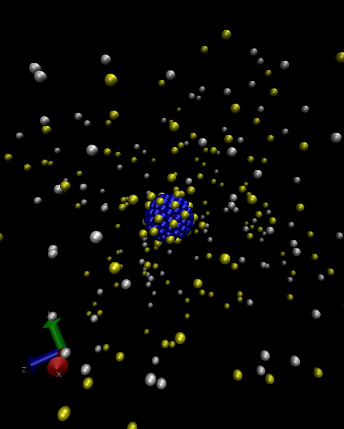
Welcome to the raspberry electrophoresis ESPResSo tutorial! This tutorial assumes some basic knowledge of ESPResSo. The first step is compiling ESPResSo with the appropriate flags, as listed in Sec. 2. The tutorial starts by discussing how to build a colloid out of a series of MD beads. These particles typically resemble a raspberry as can be seen in Fig. 1. After covering the construction of a raspberry colloid, we then briefly discuss the inclusion of hydrodynamic interactions via a lattice-Boltzmann fluid. Finally we will cover including ions via the restrictive primitive model (hard sphere ions) and the addition of an electric field to measure the electrokinetic properties. This script will run a raspberry electrophoresis simulation and write the time and position of the colloid out to a file named posVsTime.dat in the same directory. A sample set of data is included in the file posVsTime_sample.dat.
The first thing to do with any ESPResSo project is to compile ESPResSo with all of the necessary features. The following myconfig.hpp example contains all of the flags needed for running the accompanying Python script. Please compile ESPResSo using this myconfig.hpp before starting this tutorial.
#define ELECTROSTATICS
#define ROTATION
#define ROTATIONAL_INERTIA
#define EXTERNAL_FORCES
#define MASS
#define VIRTUAL_SITES_RELATIVE
#define LENNARD_JONES
The first thing to do in any ESPResSo simulation is to import our espressomd features and set a few global simulation parameters:
import espressomd
espressomd.assert_features(["ELECTROSTATICS", "ROTATION", "ROTATIONAL_INERTIA", "EXTERNAL_FORCES",
                            "MASS", "VIRTUAL_SITES_RELATIVE", "CUDA", "LENNARD_JONES"])
from espressomd import interactions
from espressomd import electrostatics
from espressomd import lb
from espressomd.virtual_sites import VirtualSitesRelative

import sys
import numpy as np


# Print enabled features
print(espressomd.features())

# System parameters
#############################################################
box_l = 40.  # size of the simulation box

skin = 0.3  # Skin parameter for the Verlet lists
time_step = 0.01
eq_tstep = 0.001

n_cycle = 1000
integ_steps = 150

# Interaction parameters (Lennard-Jones for raspberry)
#############################################################
radius_col = 3.
harmonic_radius = 3.0

# the subscript c is for colloid and s is for salt (also used for the surface beads)
eps_ss = 1.   # LJ epsilon between the colloid's surface particles.
sig_ss = 1.   # LJ sigma between the colloid's surface particles.
eps_cs = 48.  # LJ epsilon between the colloid's central particle and surface particles.
sig_cs = radius_col  # LJ sigma between the colloid's central particle and surface particles (colloid's radius).
a_eff = 0.32  # effective hydrodynamic radius of a bead due to the discreteness of LB.

# System setup
#############################################################
system = espressomd.System(box_l=[box_l] * 3)
system.set_random_state_PRNG()
system.time_step = time_step
['ADDITIONAL_CHECKS', 'AFFINITY', 'BMHTF_NACL', 'BOND_CONSTRAINT', 'BUCKINGHAM', 'COLLISION_DETECTION', 'CUDA', 'DIPOLAR_BARNES_HUT', 'DIPOLAR_DIRECT_SUM', 'DIPOLES', 'DP3M', 'DPD', 'EK_BOUNDARIES', 'ELECTROKINETICS', 'ELECTROSTATICS', 'ENGINE', 'EXCLUSIONS', 'EXPERIMENTAL_FEATURES', 'EXTERNAL_FORCES', 'FFTW', 'GAUSSIAN', 'GAY_BERNE', 'GSL', 'H5MD', 'HAT', 'HERTZIAN', 'LANGEVIN_PER_PARTICLE', 'LB_BOUNDARIES', 'LB_BOUNDARIES_GPU', 'LB_ELECTROHYDRODYNAMICS', 'LENNARD_JONES', 'LENNARD_JONES_GENERIC', 'LJCOS', 'LJCOS2', 'LJGEN_SOFTCORE', 'MASS', 'MEMBRANE_COLLISION', 'METADYNAMICS', 'MMM1D_GPU', 'MORSE', 'NPT', 'P3M', 'PARTICLE_ANISOTROPY', 'ROTATION', 'ROTATIONAL_INERTIA', 'SMOOTH_STEP', 'SOFT_SPHERE', 'TABULATED', 'THOLE', 'VIRTUAL_SITES', 'VIRTUAL_SITES_INERTIALESS_TRACERS', 'VIRTUAL_SITES_RELATIVE', 'WCA']
The parameter box_l sets the size of the simulation box. In general, one should check for finite size effects which can be surprisingly large in simulations using hydrodynamic interactions. They also generally scale as box_l$^{-1}$ or box_l$^{-3}$ depending on the transport mechanism which sometimes allows for the infinite box limit to be extrapolated to, instead of using an excessively large simulation box. As a rule of thumb, the box size should be five times greater than the characteristic length scale of the object. Note that this example uses a small box to provide a shorter simulation time.
system.cell_system.skin = skin
The skin is used for constructing the Verlet lists and is purely an optimization parameter. Whatever value provides the fastest integration speed should be used. For the type of simulations covered in this tutorial, this value turns out to be skin$\ \approx 0.3$.
system.periodicity = [True, True, True]
The periodicity parameter indicates that the system is periodic in all three dimensions. Note that the lattice-Boltzmann algorithm requires periodicity in all three directions (although this can be modified using boundaries, a topic not covered in this tutorial).
Setting up the raspberry is a non-trivial task. The main problem lies in creating a relatively uniform distribution of beads on the surface of the colloid. In general one should take about 1 bead per lattice-Boltzmann grid point on the surface to ensure that there are no holes in the surface. The behavior of the colloid can be further improved by placing beads inside the colloid, though this is not done in this example script. In our example we first define a harmonic interaction causing the surface beads to be attracted to the center, and a Lennard-Jones interaction preventing the beads from entering the colloid. There is also a Lennard-Jones potential between the surface beads to get them to distribute evenly on the surface.
# the LJ potential with the central bead keeps all the beads from simply collapsing into the center
system.non_bonded_inter[1, 0].lennard_jones.set_params(
    epsilon=eps_cs, sigma=sig_cs,
    cutoff=sig_cs * np.power(2., 1. / 6.), shift="auto")
# the LJ potential (WCA potential) between surface beads causes them to be roughly equidistant on the
# colloid surface
system.non_bonded_inter[1, 1].lennard_jones.set_params(
    epsilon=eps_ss, sigma=sig_ss,
    cutoff=sig_ss * np.power(2., 1. / 6.), shift="auto")

# the harmonic potential pulls surface beads towards the central colloid bead
col_center_surface_bond = interactions.HarmonicBond(k=3000., r_0=harmonic_radius)
system.bonded_inter.add(col_center_surface_bond)
We set up the central bead and the other beads are initialized at random positions on the surface of the colloid. The beads are then allowed to relax using an integration loop where the forces between the beads are capped.
# for the warmup we use a Langevin thermostat with an extremely low temperature and high friction coefficient
# such that the trajectories roughly follow the gradient of the potential while not accelerating too much
system.thermostat.set_langevin(kT=0.00001, gamma=40., seed=42)

print("# Creating raspberry")
center = system.box_l / 2
colPos = center

# Charge of the colloid
q_col = -40
# Number of particles making up the raspberry (surface particles + the central particle).
n_col_part = int(4 * np.pi * np.power(radius_col, 2) + 1)

# Place the central particle
system.part.add(id=0, pos=colPos, type=0, q=q_col, fix=(1, 1, 1),
                rotation=(1, 1, 1))  # Create central particle

# Create surface beads uniformly distributed over the surface of the central particle
for i in range(1, n_col_part):
    colSurfPos = np.random.randn(3)
    colSurfPos = colSurfPos / np.linalg.norm(colSurfPos) * radius_col + colPos
    system.part.add(id=i, pos=colSurfPos, type=1)
    system.part[i].add_bond((col_center_surface_bond, 0))
print("# Number of colloid beads = {}".format(n_col_part))

# Relax bead positions. The LJ potential with the central bead combined with the
# harmonic bond keep the monomers roughly radius_col away from the central bead. The LJ
# between the surface beads cause them to distribute more or less evenly on the surface.
system.force_cap = 1000
system.time_step = eq_tstep

print("Relaxation of the raspberry surface particles")
for i in range(n_cycle):
    system.integrator.run(integ_steps)

# Restore time step
system.time_step = time_step
# Creating raspberry
# Number of colloid beads = 114
Relaxation of the raspberry surface particles
The best way to ensure a relatively uniform distribution of the beads on the surface is to simply take a look at a VMD snapshot of the system after this integration. Such a snapshot is shown in Fig. 1.
In order to make the colloid perfectly round, we now adjust the bead's positions to be exactly radius_col away from the central bead.
# this loop moves the surface beads such that they are once again exactly radius_col away from the center
# For the scalar distance, we use system.distance() which considers periodic boundaries
# and the minimum image convention
colPos = system.part[0].pos
for p in system.part[1:]:
    p.pos = (p.pos - colPos) / np.linalg.norm(system.distance(p, system.part[0])) * radius_col + colPos
    p.pos = (p.pos - colPos) / np.linalg.norm(p.pos - colPos) * radius_col + colPos
Now that the beads are arranged in the shape of a raspberry, the surface beads are made virtual particles using the VirtualSitesRelative scheme. This converts the raspberry to a rigid body in which the surface particles follow the translation and rotation of the central particle. Newton's equations of motion are only integrated for the central particle. It is given an appropriate mass and moment of inertia tensor (note that the inertia tensor is given in the frame in which it is diagonal.)
# Select the desired implementation for virtual sites
system.virtual_sites = VirtualSitesRelative(have_velocity=True)
# Setting min_global_cut is necessary when there is no interaction defined with a range larger than
# the colloid such that the virtual particles are able to communicate their forces to the real particle
# at the center of the colloid
system.min_global_cut = radius_col

# Calculate the center of mass position (com) and the moment of inertia (momI) of the colloid
com = np.average(system.part[1:].pos, 0)  # system.part[:].pos returns an n-by-3 array
momI = 0
for i in range(n_col_part):
    momI += np.power(np.linalg.norm(com - system.part[i].pos), 2)

# note that the real particle must be at the center of mass of the colloid because of the integrator
print("\n# moving central particle from {} to {}".format(system.part[0].pos, com))
system.part[0].fix = 0, 0, 0
system.part[0].pos = com
system.part[0].mass = n_col_part
system.part[0].rinertia = np.ones(3) * momI

# Convert the surface particles to virtual sites related to the central particle
# The id of the central particles is 0, the ids of the surface particles start at 1.
for p in system.part[1:]:
    p.vs_auto_relate_to(0)
# moving central particle from [20. 20. 20.] to [19.99963846 20.00058187 20.00257724]
Next we insert enough ions at random positions (outside the radius of the colloid) with opposite charge to the colloid such that the system is electro-neutral. In addition, ions of both signs are added to represent the salt in the solution.
print("# Adding the positive ions")
salt_rho = 0.001  # Number density of ions
volume = system.volume()
N_counter_ions = int(round((volume * salt_rho) + abs(q_col)))

i = 0
while i < N_counter_ions:
    pos = np.random.random(3) * system.box_l
    # make sure the ion is placed outside of the colloid
    if (np.power(np.linalg.norm(pos - center), 2) > np.power(radius_col, 2) + 1):
        system.part.add(pos=pos, type=2, q=1)
        i += 1

print("# Added {} positive ions".format(N_counter_ions))

print("\n# Adding the negative ions")

N_co_ions = N_counter_ions - abs(q_col)
i = 0
while i < N_co_ions:
    pos = np.random.random(3) * system.box_l
    # make sure the ion is placed outside of the colloid
    if (np.power(np.linalg.norm(pos - center), 2) > np.power(radius_col, 2) + 1):
        system.part.add(pos=pos, type=3, q=-1)
        i += 1

print("# Added {} negative ions".format(N_co_ions))
# Adding the positive ions
# Added 104 positive ions

# Adding the negative ions
# Added 64 negative ions
We then check that charge neutrality is maintained
# Check charge neutrality
assert np.abs(np.sum(system.part[:].q)) < 1E-10
A WCA potential acts between all of the ions. This potential represents a purely repulsive version of the Lennard-Jones potential, which approximates hard spheres of diameter $\sigma$. The ions also interact through a WCA potential with the central bead of the colloid, using an offset of around $\mathrm{radius\_col}-\sigma +a_\mathrm{grid}/2$. This makes the colloid appear as a hard sphere of radius roughly $\mathrm{radius\_col}+a_\mathrm{grid}/2$ to the ions, which is approximately equal to the hydrodynamic radius of the colloid
# WCA interactions for the ions, essentially giving them a finite volume
system.non_bonded_inter[0, 2].lennard_jones.set_params(
    epsilon=eps_ss, sigma=sig_ss,
    cutoff=sig_ss * pow(2., 1. / 6.), shift="auto", offset=sig_cs - 1 + a_eff)
system.non_bonded_inter[0, 3].lennard_jones.set_params(
    epsilon=eps_ss, sigma=sig_ss,
    cutoff=sig_ss * pow(2., 1. / 6.), shift="auto", offset=sig_cs - 1 + a_eff)
system.non_bonded_inter[2, 2].lennard_jones.set_params(
    epsilon=eps_ss, sigma=sig_ss,
    cutoff=sig_ss * pow(2., 1. / 6.), shift="auto")
system.non_bonded_inter[2, 3].lennard_jones.set_params(
    epsilon=eps_ss, sigma=sig_ss,
    cutoff=sig_ss * pow(2., 1. / 6.), shift="auto")
system.non_bonded_inter[3, 3].lennard_jones.set_params(
    epsilon=eps_ss, sigma=sig_ss,
    cutoff=sig_ss * pow(2., 1. / 6.), shift="auto")
After inserting the ions, again a short integration is performed with a force cap to prevent strong overlaps between the ions.
print("\n# Equilibrating the ions (without electrostatics):")
# Langevin thermostat for warmup before turning on the LB.
temperature = 1.0
system.thermostat.set_langevin(kT=temperature, gamma=1.)

print("Removing overlap between ions")
ljcap = 100
CapSteps = 100
for i in range(CapSteps):
    system.force_cap = ljcap
    system.integrator.run(integ_steps)
    ljcap += 5

system.force_cap = 0
# Equilibrating the ions (without electrostatics):
Removing overlap between ions
Electrostatics are simulated using the Particle-Particle Particle-Mesh (P3M) algorithm. In ESPResSo this can be added to the simulation rather trivially:
# Turning on the electrostatics
# Note: Production runs would typically use a target accuracy of 10^-4
print("\n# p3m starting...")
bjerrum = 2.
p3m = electrostatics.P3M(prefactor=bjerrum * temperature, accuracy=0.001)
system.actors.add(p3m)
print("# p3m started!")
# p3m starting...
P3M tune parameters: Accuracy goal = 1.00000e-03 prefactor = 2.00000e+00
System: box_l = 4.00000e+01 # charged part = 169 Sum[q_i^2] = 1.76800e+03
mesh cao r_cut_iL     alpha_L      err          rs_err     ks_err     time [ms]
6    7   cao too large for this mesh
10   7   4.20356e-01 6.11568e+00 9.98646e-04 7.071e-04 7.052e-04 0.75
10   6   4.39595e-01 5.83813e+00 9.96988e-04 7.071e-04 7.028e-04 0.66
10   5   4.74224e-01 5.39622e+00 9.98611e-04 7.071e-04 7.051e-04 0.60
10   4   4.92500e-01 5.18846e+00 1.59302e-03 7.071e-04 1.427e-03 accuracy not achieved
14   5   3.51037e-01 7.37311e+00 9.90411e-04 7.071e-04 6.935e-04 0.68
14   4   4.13093e-01 6.22732e+00 9.98795e-04 7.071e-04 7.054e-04 0.64
14   6   3.24176e-01 8.00771e+00 9.93573e-04 7.071e-04 6.980e-04 0.56
14   7   3.10283e-01 8.37985e+00 9.94792e-04 7.071e-04 6.997e-04 0.65
18   6   2.57695e-01 1.01590e+01 9.95660e-04 7.071e-04 7.010e-04 0.84
18   5   2.79855e-01 9.32636e+00 9.91451e-04 7.071e-04 6.950e-04 0.77
18   7   2.46931e-01 1.06183e+01 9.89337e-04 7.071e-04 6.919e-04 0.91
18   4   3.24176e-01 8.00771e+00 1.06800e-03 7.071e-04 8.004e-04 accuracy not achieved
22   6   2.14811e-01 1.22677e+01 9.89855e-04 7.071e-04 6.927e-04 1.11
22   5   2.33395e-01 1.12571e+01 9.94381e-04 7.071e-04 6.991e-04 1.04
22   7   2.05519e-01 1.28428e+01 9.87214e-04 7.071e-04 6.889e-04 1.20
22   4   2.78216e-01 9.38335e+00 9.96582e-04 7.071e-04 7.023e-04 1.03
22   3   2.79855e-01 9.32636e+00 3.37644e-03 7.071e-04 3.302e-03 accuracy not achieved
26   6   1.84209e-01 1.43847e+01 9.94692e-04 7.071e-04 6.996e-04 1.61
26   5   2.00511e-01 1.31752e+01 9.99588e-04 7.071e-04 7.065e-04 1.55
26   7   1.76058e-01 1.50748e+01 9.93849e-04 7.071e-04 6.984e-04 1.75
26   4   2.40178e-01 1.09279e+01 9.98437e-04 7.071e-04 7.049e-04 1.50
26   3   2.78216e-01 9.38335e+00 2.03967e-03 7.071e-04 1.913e-03 accuracy not achieved
30   6   1.62308e-01 1.63991e+01 9.74711e-04 7.071e-04 6.709e-04 2.22
30   5   1.76381e-01 1.50463e+01 9.96803e-04 7.071e-04 7.026e-04 2.12
30   7   1.54802e-01 1.72229e+01 9.77837e-04 7.071e-04 6.754e-04 2.36
30   4   2.12032e-01 1.24343e+01 9.96452e-04 7.071e-04 7.021e-04 2.06
30   3   2.40178e-01 1.09279e+01 2.24420e-03 7.071e-04 2.130e-03 accuracy not achieved
34   6   1.44116e-01 1.85465e+01 9.95170e-04 7.071e-04 7.003e-04 5.52
34   5   1.58196e-01 1.68406e+01 9.81989e-04 7.071e-04 6.814e-04 5.15
34   7   1.37490e-01 1.94723e+01 9.95838e-04 7.071e-04 7.012e-04 5.35
34   4   1.90498e-01 1.38932e+01 9.89537e-04 7.071e-04 6.922e-04 6.34
34   3   2.12032e-01 1.24343e+01 2.40867e-03 7.071e-04 2.303e-03 accuracy not achieved

resulting parameters: mesh: (14 14 14), cao: 6, r_cut_iL: 3.2418e-01,
                      alpha_L: 8.0077e+00, accuracy: 9.9357e-04, time: 0.56

# p3m started!
Generally a Bjerrum length of $2$ is appropriate when using WCA interactions with $\sigma=1$, since a typical ion has a radius of $0.35\ \mathrm{nm}$, while the Bjerrum length in water is around $0.7\ \mathrm{nm}$.
The external electric field is simulated by simply adding a constant force equal to the simulated field times the particle charge. Generally the electric field is set to $0.1$ in MD units, which is the maximum field before the response becomes nonlinear. Smaller fields are also possible, but the required simulation time is considerably larger. Sometimes, Green-Kubo methods are also used, but these are generally only feasible in cases where there is either no salt or a very low salt concentration.
Efield = np.array((0.1, 0, 0)) # an electric field of 0.1 is the upper limit of the linear response regime for this model
for p in system.part:
    p.ext_force = p.q * Efield
Before creating the LB fluid it is a good idea to set all of the particle velocities to zero. This is necessary to set the total momentum of the system to zero. Failing to do so will lead to an unphysical drift of the system, which will change the values of the measured velocities.
system.part[:].v = (0, 0, 0)
The important parameters for the LB fluid are the density, the viscosity, the time step, and the friction coefficient used to couple the particle motion to the fluid. The time step should generally be comparable to the MD time step. While large time steps are possible, a time step of $0.01$ turns out to provide more reasonable values for the root mean squared particle velocities. Both density and viscosity should be around $1$, while the friction should be set around $20.$ The grid spacing should be comparable to the ions' size.
lb=espressomd.lb.LBFluidGPU(kT=temperature, seed=42, dens=1., visc=3., agrid=1., tau=system.time_step)
system.actors.add(lb)
A logical way of picking a specific set of parameters is to choose them such that the hydrodynamic radius of an ion roughly matches its physical radius determined by the WCA potential ($R=0.5\sigma$). Using the following equation:
\begin{equation} \frac{1}{\Gamma}=\frac{1}{6\pi \eta R_{\mathrm{H0}}}=\frac{1}{\Gamma_0} +\frac{1}{g\eta a} \label{effectiveGammaEq} \end{equation}one can see that the set of parameters grid spacing $a=1\sigma$, fluid density $\rho=1$, a kinematic viscosity of $\nu=3 $ and a friction of $\Gamma_0=50$ leads to a hydrodynamic radius of approximately $0.5\sigma$.
The last step is to first turn off all other thermostats, followed by turning on the LB thermostat. The temperature is typically set to 1, which is equivalent to setting $k_\mathrm{B}T=1$ in molecular dynamics units.
system.thermostat.turn_off()
system.thermostat.set_lb(LB_fluid=lb, seed=123, gamma=20.0)
Now the main simulation can begin! The only important thing is to make sure the system has enough time to equilibrate. There are two separate equilibration times: 1) the time for the ion distribution to stabilize, and 2) the time needed for the fluid flow profile to equilibrate. In general, the ion distribution equilibrates fast, so the needed warmup time is largely determined by the fluid relaxation time, which can be calculated via $\tau_\mathrm{relax} = \mathrm{box\_length}^2/\nu$. This means for a box of size 40 with a kinematic viscosity of 3 as in our example script, the relaxation time is $\tau_\mathrm{relax} = 40^2/3 = 533 \tau_\mathrm{MD}$, or 53300 integration steps. In general it is a good idea to run for many relaxation times before starting to use the simulation results for averaging observables. To be on the safe side $10^6$ integration steps is a reasonable equilibration time. Please feel free to modify the provided script and try and get some interesting results!
# Reset the simulation clock
system.time = 0
initial_pos = system.part[0].pos
num_iterations = 20
num_steps_per_iteration = 1000
posVsTime = open('posVsTime.dat', 'w')  # file where the raspberry position will be written

for i in range(num_iterations):
    system.integrator.run(num_steps_per_iteration)
    pos = system.part[0].pos - initial_pos
    posVsTime.write("%.2f %.4f %.4f %.4f\n" % (system.time, pos[0], pos[1], pos[2]))
    posVsTime.flush()
    print("# time: {:.0f}, col_pos: {}".format(system.time, pos))

posVsTime.close()

print("\n# Finished")
# time: 10, col_pos: [0.12139151 0.33648271 0.11251692]
# time: 20, col_pos: [ 0.26465217  0.22024054 -0.78458   ]
# time: 30, col_pos: [ 0.50993049  0.45817406 -0.84871356]
# time: 40, col_pos: [ 0.663389    0.44962719 -0.91640851]
# time: 50, col_pos: [ 0.34887608  0.13742542 -1.01495835]
# time: 60, col_pos: [ 0.53370487  0.17153412 -1.06349154]
# time: 70, col_pos: [ 1.0077143   0.14453912 -1.02910501]
# time: 80, col_pos: [ 1.20528906 -0.09712912 -0.97491627]
# time: 90, col_pos: [ 1.27609946  0.16715651 -1.29569826]
# time: 100, col_pos: [ 1.32131969  0.45387204 -1.27172271]
# time: 110, col_pos: [ 1.33615426  0.60632134 -1.11445053]
# time: 120, col_pos: [ 0.71272482  0.46151833 -1.08936277]
# time: 130, col_pos: [ 0.68442417  0.78635935 -1.09995237]
# time: 140, col_pos: [ 0.49086562  0.76510262 -0.7781581 ]
# time: 150, col_pos: [ 0.80720067  0.76006062 -0.61366391]
# time: 160, col_pos: [ 0.85798905  0.77378094 -0.66713013]
# time: 170, col_pos: [ 0.74651213  1.29441379 -0.9816953 ]
# time: 180, col_pos: [ 0.44918504  1.2117107  -0.9135223 ]
# time: 190, col_pos: [ 0.4484768   0.74848315 -1.61077491]
# time: 200, col_pos: [ 0.33371897  0.84318472 -1.61429722]

# Finished