3. Running a simulation
ESPResSo is implemented as a Python module. This means that you need to write a python script for any task you want to perform with ESPResSo. In this chapter, the basic structure of the interface will be explained. For a practical introduction, see the tutorials, which are also part of the distribution.
3.1. Running ESPResSo
3.1.1. Running a script
To use ESPResSo, you need to import the espressomd module in your
Python script. To this end, the folder containing the python module
needs to be in the Python search path. The module is located in the
src/python folder under the build directory.
A convenient way to run Python with the correct path is to use the
pypresso script located in the build directory:
./pypresso simulation.py
The pypresso script is just a wrapper in order to expose the ESPResSo python
module to the system’s Python interpreter by modifying the $PYTHONPATH.
If you have installed ESPResSo from a Linux package manager that doesn’t provide
the pypresso script, you will need to modify the $PYTHONPATH and
possibly the $LD_LIBRARY_PATH too, depending on which symbols are missing.
The next chapter, Setting up the system, will explain in more details how to write a simulation script for ESPResSo. If you don’t have any script, simply call one of the files listed in section Sample scripts.
3.1.2. Using the console
Since ESPResSo can be manipulated like any other Python module, it is possible
to interact with it in a Python interpreter. Simply run the pypresso
script without arguments to start a Python session:
./pypresso
Likewise, a Jupyter console can be started with the ipypresso script,
which is also located in the build directory:
./ipypresso console
The name comes from the IPython interpreter, today known as Jupyter.
3.1.3. Interactive notebooks
Tutorials are available as notebooks, i.e. they consist of a .ipynb
file which contains both the source code and the corresponding explanations.
They can be viewed, changed and run interactively. To generate the tutorials
in the build folder, do:
make tutorials
The tutorials contain solutions hidden with the exercise2 NB extension.
Since this extension is only available for Jupyter Notebook, JupyterLab
users need to convert the tutorials:
for f in doc/tutorials/*/*.ipynb; do
  ./pypresso doc/tutorials/convert.py exercise2 --to-jupyterlab ${f}
done
To interact with notebooks, move to the directory containing the tutorials
and call the ipypresso script to start a local Jupyter session.
For Jupyter Notebook and IPython users:
cd doc/tutorials
../../ipypresso notebook
For JupyterLab users:
cd doc/tutorials
../../ipypresso lab
You may then browse through the different tutorial folders. Files whose name
ends with extension .ipynb can be opened in the browser. Click on the Run
button to execute the current block, or use the keyboard shortcut Shift+Enter.
If the current block is a code block, the In [ ] label to the left will
change to In [*] while the code is being executed, and become In [1]
once the execution has completed. The number increments itself every time a
code cell is executed. This bookkeeping is extremely useful when modifying
previous code cells, as it shows which cells are out-of-date. It’s also
possible to run all cells by clicking on the “Run” drop-down menu, then on
“Run All Below”. This will change all labels to In [*] to show that the
first one is running, while the subsequent ones are awaiting execution.
You’ll also see that many cells generate an output. When the output becomes very long, Jupyter will automatically put it in a box with a vertical scrollbar. The output may also contain static plots, dynamic plots and videos. It is also possible to start a 3D visualizer in a new window, however closing the window will exit the Python interpreter and Jupyter will notify you that the current Python kernel stopped. If a cell takes too long to execute, you may interrupt it with the stop button.
Solutions cells are created using the exercise2 plugin from nbextensions.
To prevent solution code cells from running when clicking on “Run All”, these
code cells need to be converted to Markdown cells and fenced with ```python
and ```.
To close the Jupyter session, go to the terminal where it was started and use the keyboard shortcut Ctrl+C twice.
When starting a Jupyter session, you may see the following warning in the terminal:
[TerminalIPythonApp] WARNING | Subcommand `ipython notebook` is deprecated and will be removed in future versions.
[TerminalIPythonApp] WARNING | You likely want to use `jupyter notebook` in the future
This only means ESPResSo was compiled with IPython instead of Jupyter. If Jupyter
is installed on your system, the notebook will automatically close IPython and
start Jupyter. To recompile ESPResSo with Jupyter, provide cmake with the flag
-DIPYTHON_EXECUTABLE=$(which jupyter).
You can find the official Jupyter documentation at https://jupyter.readthedocs.io/en/latest/running.html
3.1.4. Running inside an IDE
You can use an integrated development environment (IDE) to develop and run ESPResSo scripts. Suitable IDEs are e.g. Visual Studio Code and Spyder. They can provide a workflow superior to that of a standard text editor as they offer useful features such as advanced code completion, debugging and analysis tools etc. The following example shows how to setup ESPResSo in Visual Studio Code on Linux (tested with version 1.46.1). The process should be similar for every Python IDE, namely the Python interpreter needs to be replaced.
The pypresso executable can be set as a custom Python interpreter inside VS
Code. ESPResSo scripts can then be executed just like any other python script.
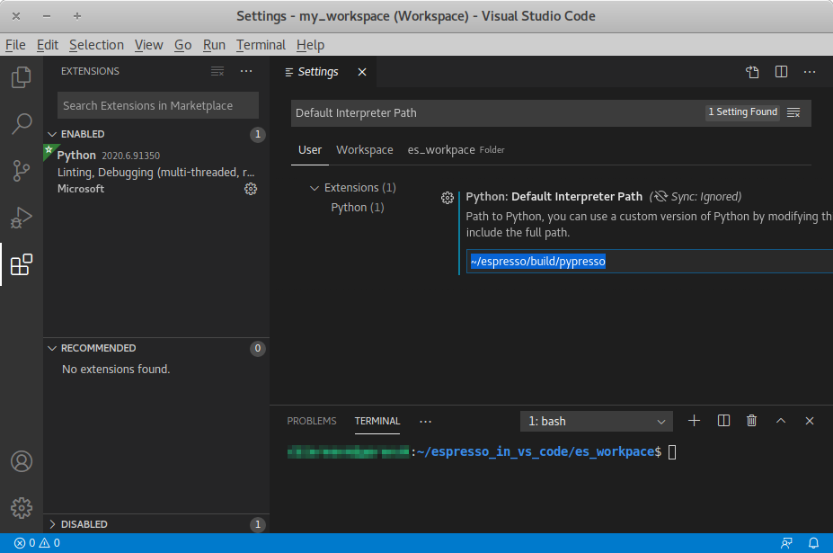
Inside VS Code, the Python extension needs to be installed. Next, click the
gear at the bottom left and choose Settings. Search for
Default Interpreter Path and change the setting to the path to your
pypresso executable, e.g.
~/espresso/build/pypresso
After that, you can open scripts and execute them with the keyboard shortcut Ctrl+F5.
Fig. Visual Studio Code interface shows the VS Code interface with the interpreter
path set to pypresso.
Note
You may need to set the path relative to your home directory, i.e. ~/path/to/pypresso.
Visual Studio Code interface
3.2. Debugging ESPResSo
Exceptional situations occur in every program. If ESPResSo crashes with a
segmentation fault, that means that there was a memory fault in the
simulation core which requires running the program in a debugger. The
pypresso executable file is actually not a program but a script
which sets the Python path appropriately and starts the Python
interpreter with your arguments. Thus it is not possible to directly
run pypresso in a debugger. However, we provide some useful
command line options for the most common tools.
./pypresso --tool <args>
where --tool can be any tool from the table below.
Only one tool can be used at a time. Some tools benefit from specific build
options, as outlined in the installation section Troubleshooting.
ESPResSo can be debugged in MPI environments, as outlined in section
Debugging parallel code.
Tool |
Effect |
|---|---|
|
|
|
|
|
|
|
|
|
|
3.3. Parallel computing
Many algorithms in ESPResSo are designed to work with multiple MPI ranks. However, not all algorithms benefit from MPI parallelization equally. Several algorithms only use MPI rank 0 (e.g. Reaction methods), while a small subset simply don’t support MPI (e.g. Dipolar direct sum). ESPResSo should work with most MPI implementations on the market; see the MPI installation requirements for details.
3.3.1. General syntax
To run a simulation on several MPI ranks, for example 4, simply invoke
the pypresso script with the following syntax:
mpiexec -n 4 ./pypresso simulation.py
The cell system is automatically split among the MPI ranks, and data
is automatically gathered on the main rank, which means a regular ESPResSo
script can be executed in an MPI environment out-of-the-box. The number
of MPI ranks can be accessed via the system n_nodes state property.
The simulation box partition is controlled by the cell system
node_grid property.
By default, MPI ranks are assigned in decreasing order, e.g. on 6 MPI ranks
node_grid is [3, 2, 1]. It is possible to re-assign the ranks by
changing the value of the node_grid property, however a few algorithms
(such as FFT-based electrostatic methods) only work for the default
partitioning scheme where values must be arranged in decreasing order.
# get the number of ranks
print(system.cell_system.get_state()["n_nodes"])
# re-assign the ranks
system.cell_system.node_grid = [2, 1, 3]
system.cell_system.node_grid = [6, 1, 1]
There are alternative ways to invoke MPI on pypresso, but they share
similar options. The number after the -n option is the number of ranks,
which needs to be inferior or equal to the number of physical cores on the
workstation. Command nproc displays the number of logical cores on the
workstation. For architectures that support hyperthreading, the number of
logical cores is an integer multiple of the number of physical cores,
usually 2. Therefore on a hyperthreaded workstation with 32 cores,
at most 16 cores can be used without major performance loss, unless
extra arguments are passed to the mpiexec program.
On cluster computers, it might be necessary to load the MPI library with
module load openmpi or similar.
3.3.2. Performance gain
Simulations executed in parallel with run faster, however the runtime won’t decrease linearly with the number of MPI ranks. MPI-parallel simulations introduce several sources of overhead and latency:
overhead of serializing, communicating and deserializing data structures
extra calculations in the LB halo
extra calculations in the ghost shell (see section Internal particle organization for more details)
latency due to blocking communication (i.e. a node remains idle while waiting for a message from another node)
latency due to blocking data collection for GPU (only relevant for GPU methods)
latency due to context switching
latency due to memory bandwidth
While good performance can be achieved up to 32 MPI ranks, allocating more than 32 ranks to a simulation will not always lead to significantly improved run times. The performance gain is highly sensitive to the algorithms used by the simulation, for example GPU methods rarely benefit from more than 8 MPI ranks. Performance is also affected by the number of features enabled at compile time, even when these features are not used by the simulation; do not hesitate to remove all features not required by the simulation script and rebuild ESPResSo for optimal performance.
Benchmarking is often the best way to determine the optimal number of MPI ranks for a given simulation setup. Please refer to the wiki chapter on benchmarking for more details.
Runtime speed-up is not the only appeal of MPI parallelization. Another benefit is the possibility to distribute a calculation over multiple compute nodes in clusters and high-performance environments, and therefore split the data structures over multiple machines. This becomes necessary when running simulations with millions of particles, as the memory available on a single compute node would otherwise saturate.
3.3.3. Communication model
ESPResSo was originally designed for the “flat” model of communication: each MPI rank binds to a logical CPU core. This communication model doesn’t fully leverage shared memory on recent CPUs, such as NUMA architectures, and ESPResSo currently doesn’t support the hybrid MPI+OpenMP programming model.
The MPI+CUDA programming model is supported, although only one GPU can be used for the entire simulation. As a result, a blocking gather operation is carried out to collect data from all ranks to the main rank, and a blocking scatter operation is carried out to transfer the result of the GPU calculation from the main rank back to all ranks. This latency limits GPU-acceleration to simulations running on fewer than 8 MPI ranks. For more details, see section GPU acceleration.
3.3.3.1. The MPI callbacks framework
When starting a simulation with \(n\) MPI ranks, ESPResSo will internally use MPI rank \(0\) as the head node (also referred to as the “main rank”) and MPI ranks \(1\) to \(n-1\) as worker nodes. The Python interface interacts only with the head node, and the head node forwards the information to the worker nodes.
To put it another way, all worker nodes are idle until the user calls a function that is designed to run in parallel, in which case the head node calls the corresponding core function and sends a request on the worker nodes to call the same core function. The request can be a simple collective call, or a collective call with a reduction if the function returns a value. The reduction can either:
combine the \(n\) results via a mathematical operation (usually a summation or a multiplication)
discard the result of the \(n-1\) worker nodes; this is done when all ranks return the same value, or when the calculation can only be carried out on the main rank but requires data from the other ranks
return the result of one rank when the calculation can only be carried out by a specific rank; this is achieved by returning an optional, which contains a value on the rank that has access to the information necessary to carry out the calculation, while the other \(n-1\) ranks return an empty optional
For more details on this framework, please refer to the Doxygen documentation
of the the C++ core file MpiCallbacks.hpp.
3.3.4. Debugging parallel code
It is possible to debug an MPI-parallel simulation script with GDB.
Keep in mind that contrary to a textbook example MPI application, where
all ranks execute the main function, in ESPResSo the worker nodes are idle
until the head node on MPI rank 0 delegates work to them. This means that
on MPI rank > 1, break points will only have an effect in code that can be
reached from a callback function whose pointer has been registered in the
MPI callbacks framework.
The following command runs a script with 2 MPI ranks and binds a terminal to each rank:
mpiexec -np 2 xterm -fa 'Monospace' -fs 12 -e ./pypresso --gdb simulation.py
It can also be done via ssh with X-window forwarding:
ssh -X username@hostname
mpiexec -n 2 -x DISPLAY="${DISPLAY}" xterm -fa 'Monospace' -fs 12 \
    -e ./pypresso --gdb simulation.py
The same syntax is used for C++ unit tests:
mpiexec -np 2 xterm -fa 'Monospace' -fs 12 \
    -e gdb src/core/unit_tests/EspressoSystemStandAlone_test
3.4. GPU acceleration
3.4.1. CUDA acceleration
Note
Feature CUDA required
ESPResSo is capable of delegating work to the GPU to speed up simulations. Not every simulation method profits from GPU acceleration. Refer to Available simulation methods to check whether your desired method can be used on the GPU. In order to use GPU acceleration you need a NVIDIA GPU and it needs to have at least compute capability 2.0. For more details, please refer to the installation section Nvidia GPU acceleration.
For more information please check espressomd.cuda_init.CudaInitHandle.
3.4.1.1. List available devices
To list available CUDA devices, call
espressomd.cuda_init.CudaInitHandle.list_devices():
>>> import espressomd
>>> system = espressomd.System(box_l=[1, 1, 1])
>>> print(system.cuda_init_handle.list_devices())
{0: 'GeForce RTX 2080', 1: 'GeForce GT 730'}
This method returns a dictionary containing the device id as key and the device name as its value.
To get more details on the CUDA devices for each MPI node, call
espressomd.cuda_init.CudaInitHandle.list_devices_properties():
>>> import pprint
>>> import espressomd
>>> system = espressomd.System(box_l=[1, 1, 1])
>>> pprint.pprint(system.cuda_init_handle.list_devices_properties())
{'seraue': {0: {'name': 'GeForce RTX 2080',
                'compute_capability': (7, 5),
                'cores': 46,
                'total_memory': 8370061312},
            1: {'name': 'GeForce GT 730',
                'compute_capability': (3, 5),
                'cores': 2,
                'total_memory': 1014104064}}}
3.4.1.2. Select a device
When you start pypresso, the first GPU should be selected.
If you wanted to use the second GPU, this can be done
by setting espressomd.cuda_init.CudaInitHandle.device as follows:
>>> import espressomd
>>> system = espressomd.System(box_l=[1, 1, 1])
>>> system.cuda_init_handle.device = 1
Setting a device id outside the valid range or a device which does not meet the minimum requirements will raise an exception.